Lorenz curve
In economics, the Lorenz curve is a graphical representation of the cumulative distribution function of the empirical probability distribution of wealth or income, and was developed by Max O. Lorenz in 1905 for representing inequality of the wealth distribution.
The curve is a graph showing the proportion of overall income or wealth assumed by the bottom x% of the people, although this is not rigorously true for a finite population (see below). It is often used to represent income distribution, where it shows for the bottom x% of households, what percentage (y%) of the total income they have. The percentage of households is plotted on the x-axis, the percentage of income on the y-axis. It can also be used to show distribution of assets. In such use, many economists consider it to be a measure of social inequality.
The concept is useful in describing inequality among the size of individuals in ecology[1] and in studies of biodiversity, where the cumulative proportion of species is plotted against the cumulative proportion of individuals.[2] It is also useful in business modeling: e.g., in consumer finance, to measure the actual percentage y% of delinquencies attributable to the x% of people with worst risk scores.

Explanation
Points on the Lorenz curve represent statements like "the bottom 20% of all households have 10% of the total income."
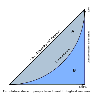
A perfectly equal income distribution would be one in which every person has the same income. In this case, the bottom N% of society would always have N% of the income. This can be depicted by the straight line y = x; called the "line of perfect equality."
By contrast, a perfectly unequal distribution would be one in which one person has all the income and everyone else has none. In that case, the curve would be at y = 0% for all x < 100%, and y = 100% when x = 100%. This curve is called the "line of perfect inequality."
The Gini coefficient is the ratio of the area between the line of perfect equality and the observed Lorenz curve to the area between the line of perfect equality and the line of perfect inequality. The higher the coefficient, the more unequal the distribution is. In the diagram on the right, this is given by the ratio A/(A+B), where A and B are the indicated areas.
Definition and calculation
The Lorenz curve can usually be represented by a function L(F), where F, the cumulative portion of the population, is represented by the horizontal axis, and L, the cumulative portion of the total wealth or income, is represented by the vertical axis.
For a population of size n, with a sequence of values yi, i = 1 to n, that are indexed in non-decreasing order ( yi ≤ yi+1), the Lorenz curve is the continuous piecewise linear function connecting the points ( Fi, Li ), i = 0 to n, where F0 = 0, L0 = 0, and for i = 1 to n:
Note that the statement that the Lorenz curve gives the portion of the wealth or income held by a given portion of the population is only strictly true at the points defined above, but not at the points on the line segments between these points. For instance, in a population of 10 households, it doesn't make sense to say that 45% of them earn a certain portion of the total. If the population is modeled as a continuum then this subtlety disappears.
For a discrete probability function f(y), let yi, i = 1 to n, be the points with non-zero probabilities indexed in increasing order ( yi < yi+1). The Lorenz curve is the continuous piecewise linear function connecting the points ( Fi, Li ), i = 0 to n, where F0 = 0, L0 = 0, and for i = 1 to n:
For a probability density function f(x) with the cumulative distribution function F(x), the Lorenz curve L(F(x)) is given by:
where  denotes the average.
For a cumulative distribution function F(x) with inverse x(F), the Lorenz curve L(F) is given by:
The inverse x(F) may not exist because the cumulative distribution function has intervals of constant values. However, the previous formula can still apply by generalizing the definition of x(F):
- x(F1) = inf {y : F(y) ≥ F1}
For an example of a Lorenz curve, see Pareto distribution.
Properties

A Lorenz curve always starts at (0,0) and ends at (1,1).
The Lorenz curve is not defined if the mean of the probability distribution is zero or infinite.
The Lorenz curve for a probability distribution is a continuous function. However, Lorenz curves representing discontinuous functions can be constructed as the limit of Lorenz curves of probability distributions, the line of perfect inequality being an example.
The information in a Lorenz curve may be summarized by the Gini coefficient and the Lorenz asymmetry coefficient.[1]
The Lorenz curve cannot rise above the line of perfect equality. If the variable being measured cannot take negative values, the Lorenz curve:
- cannot sink below the line of perfect inequality,
- is increasing.
Note however that a Lorenz curve for net worth would start out by going negative due to the fact that some people have a negative net worth because of debt.
The Lorenz curve is invariant under positive scaling. If X is a random variable, for any positive number c the random variable c X has the same Lorenz curve as X.
The Lorenz curve is flipped twice, once about F = 0.5 and once about L = 0.5, by negation. If X is a random variable with Lorenz curve LX(F), then −X has the Lorenz curve:
- L − X = 1 − L X (1 − F)
The Lorenz curve is changed by translations so that the equality gap F − L(F) changes in proportion to the ratio of the original and translated means. If X is a random variable with a Lorenz curve L X (F) and mean μ X , then for any constant c ≠ −μ X , X + c has a Lorenz curve defined by:
For a cumulative distribution function F(x) with mean μ and (generalized) inverse x(F), then for any F with 0 < F < 1 :
- If the Lorenz curve is differentiable:
- If the Lorenz curve is twice differentiable, then the probability density function f(x) exists at that point and:
- If L(F) is continuously differentiable, then the tangent of L(F) is parallel to the line of perfect equality at the point F(μ). This is also the point at which the equality gap F − L(F), the vertical distance between the Lorenz curve and the line of perfect equality, is greatest. The size of the gap is equal to half of the relative mean deviation:
See also
| Wikimedia Commons has media related to Lorenz curve. |
- Distribution (economics)
- Distribution of wealth
- Welfare economics
- Income inequality metrics
- Gini coefficient
- Hoover index (a.k.a. Robin Hood index)
- ROC analysis
- Social welfare (political science)
- Economic inequality
- Zipf's law
- Pareto distribution
- Mean deviation
References
- ↑ 1.0 1.1 Damgaard, Christian; Jacob Weiner (2000). "Describing inequality in plant size or fecundity". Ecology 81 (4): 1139–1142. doi:10.1890/0012-9658(2000)081[1139:DIIPSO]2.0.CO;2.
- ↑ Wittebolle, Lieven et al. (2009). "Initial community evenness favours functionality under selective stress". Nature 458 (7238): 623–626. Bibcode:2009Natur.458..623W. doi:10.1038/nature07840. PMID 19270679.
Further reading
- Lorenz, M. O. (1905). "Methods of measuring the concentration of wealth". Publications of the American Statistical Association (Publications of the American Statistical Association, Vol. 9, No. 70) 9 (70): 209–219. Bibcode:1905PAmSA...9..209L. doi:10.2307/2276207. JSTOR 2276207.
- Gastwirth, Joseph L. (1972). "The Estimation of the Lorenz Curve and Gini Index". The Review of Economics and Statistics (The Review of Economics and Statistics, Vol. 54, No. 3) 54 (3): 306–316. doi:10.2307/1937992. JSTOR 1937992.
- Chakravarty, S. R. (1990). Ethical Social Index Numbers. New York: Springer-Verlag. ISBN 0-387-52274-3.
- Anand, Sudhir (1983). Inequality and Poverty in Malaysia. New York: Oxford University Press. ISBN 0-19-520153-1.
External links
- WIID: World Income Inequality Database, the most comprehensive source of information on inequality, collected by WIDER (World Institute for Development Economics Research, part of United Nations University)
- glcurve: Stata module to plot Lorenz curve (type "findit glcurve" or "ssc install glcurve" in Stata prompt to install)
- Free add-on to STATA to compute inequality and poverty measures
- Free Online Software (Calculator) computes the Gini Coefficient, plots the Lorenz curve, and computes many other measures of concentration for any dataset
- Free Calculator: Online and downloadable scripts (Python and Lua) for Atkinson, Gini, and Hoover inequalities
- Users of the R data analysis software can install the "ineq" package which allows for computation of a variety of inequality indices including Gini, Atkinson, Theil.
- A MATLAB Inequality Package, including code for computing Gini, Atkinson, Theil indexes and for plotting the Lorenz Curve. Many examples are available.
- A complete handout about the Lorenz curve including various applications, including an Excel spreadsheet graphing Lorenz curves and calculating Gini coefficients as well as coefficients of variation.
- LORENZ 3.0 is a Mathematica notebook which draw sample Lorenz curves and calculates Gini coefficients and Lorenz asymmetry coefficients from data in an Excel sheet.


