Logistic regression
| Regression analysis |
|---|
 |
| Models |
| Estimation |
| Background |
|
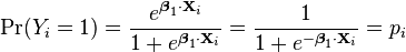
In statistics, logistic regression, or logit regression, or logit model[1] is a direct probability model that was developed by statistician D. R. Cox in 1958[2] and,[3] although much work was done in the single independent variable case almost two decades earlier. The binary logistic model is used to predict a binary response based on one or more predictor variables (features). That is, it is used in estimating the parameters of a qualitative response model. The probabilities describing the possible outcomes of a single trial are modeled, as a function of the explanatory (predictor) variables, using a logistic function. Frequently (and hereafter in this article) "logistic regression" is used to refer specifically to the problem in which the dependent variable is binary—that is, the number of available categories is two—while problems with more than two categories are referred to as multinomial logistic regression or polytomous logistic regression, or, if the multiple categories are ordered, as ordinal logistic regression.[3]
Logistic regression measures the relationship between the categorical dependent variable and one or more independent variables, which are usually (but not necessarily) continuous, by estimating probabilities. Thus, it treats the same set of problems as does probit regression using similar techniques; the first assumes a logistic function and the second a standard normal distribution function.
Logistic regression can be seen as a special case of generalized linear model and thus analogous to linear regression. The model of logistic regression, however, is based on quite different assumptions (about the relationship between dependent and independent variables) from those of linear regression. In particular the key differences of these two models can be seen in the following two features of logistic regression. First, the conditional distribution  is a Bernoulli distribution rather than a Gaussian distribution, because the dependent variable is binary. Second, the estimated probabilities are restricted to [0,1] through the logistic distribution function because logistic regression predicts the probability of the instance being positive.
Logistic regression is an alternative to Fisher's 1936 classification method, linear discriminant analysis.[4] If the assumptions of linear discriminant analysis hold, application of Bayes' rule to reverse the conditioning results in the logistic model, so if linear discriminant assumptions are true, logistic regression assumptions must hold. The converse is not true, so the logistic model has fewer assumptions than discriminant analysis and makes no assumption on the distribution of the independent variables.
Fields and example applications
Logistic regression is used widely in many fields, including the medical and social sciences. For example, the Trauma and Injury Severity Score (TRISS), which is widely used to predict mortality in injured patients, was originally developed by Boyd et al. using logistic regression.[5] Many other medical scales used to assess severity of a patient have been developed using logistic regression.[6][7][8][9] Logistic regression may be used to predict whether a patient has a given disease (e.g. diabetes; coronary heart disease), based on observed characteristics of the patient (age, sex, body mass index, results of various blood tests, etc.; age, blood cholesterol level, systolic blood pressure, relative weight, blood hemoglobin level, smoking (at 3 levels), and abnormal electrocardiogram.).[1][10] Another example might be to predict whether an American voter will vote Democratic or Republican, based on age, income, sex, race, state of residence, votes in previous elections, etc.[11] The technique can also be used in engineering, especially for predicting the probability of failure of a given process, system or product.[12][13] It is also used in marketing applications such as prediction of a customer's propensity to purchase a product or halt a subscription, etc. In economics it can be used to predict the likelihood of a person's choosing to be in the labor force, and a business application would be to predict the likelihood of a homeowner defaulting on a mortgage. Conditional random fields, an extension of logistic regression to sequential data, are used in natural language processing.
Basics
Logistic regression can be binomial or multinomial. Binomial or binary logistic regression deals with situations in which the observed outcome for a dependent variable can have only two possible types (for example, "dead" vs. "alive"). Multinomial logistic regression deals with situations where the outcome can have three or more possible types (e.g., "disease A" vs. "disease B" vs. "disease C"). In binary logistic regression, the outcome is usually coded as "0" or "1", as this leads to the most straightforward interpretation.[14] If a particular observed outcome for the dependent variable is the noteworthy possible outcome (referred to as a "success" or a "case") it is usually coded as "1" and the contrary outcome (referred to as a "failure" or a "noncase") as "0". Logistic regression is used to predict the odds of being a case based on the values of the independent variables (predictors). The odds are defined as the probability that a particular outcome is a case divided by the probability that it is a noncase.
Like other forms of regression analysis, logistic regression makes use of one or more predictor variables that may be either continuous or categorical data. Unlike ordinary linear regression, however, logistic regression is used for predicting binary outcomes of the dependent variable (treating the dependent variable as the outcome of a Bernoulli trial) rather than a continuous outcome. Given this difference, it is necessary that logistic regression take the natural logarithm of the odds of the dependent variable being a case (referred to as the logit or log-odds) to create a continuous criterion as a transformed version of the dependent variable. Thus the logit transformation is referred to as the link function in logistic regression—although the dependent variable in logistic regression is binomial, the logit is the continuous criterion upon which linear regression is conducted.[14]
The logit of success is then fitted to the predictors using linear regression analysis. The predicted value of the logit is converted back into predicted odds via the inverse of the natural logarithm, namely the exponential function. Thus, although the observed dependent variable in logistic regression is a zero-or-one variable, the logistic regression estimates the odds, as a continuous variable, that the dependent variable is a success (a case). In some applications the odds are all that is needed. In others, a specific yes-or-no prediction is needed for whether the dependent variable is or is not a case; this categorical prediction can be based on the computed odds of a success, with predicted odds above some chosen cutoff value being translated into a prediction of a success.
Logistic function, odds, odds ratio, and logit

 ; note that
 ![\sigma (t) \in [0,1]](../I/m/a1e9708e9354c2ca4a2268059e5dd029.png) for all
for all  .
.Definition of the logistic function
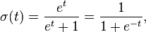
An explanation of logistic regression begins with an explanation of the logistic function. The logistic function is useful because it can take an input with any value from negative to positive infinity, whereas the output always takes values between zero and one[14] and hence is interpretable as a probability. The logistic function is defined as follows:
A graph of the logistic function is shown in Figure 1.
If is viewed as a linear function of an explanatory variable  (or of a linear combination of explanatory variables), then we express as follows:
And the logistic function can now be written as:
Note that  is interpreted as the probability of the dependent variable equaling a "success" or "case" rather than a failure or non-case. It's clear that the response variables
  are not identically distributed:
  differs from one data point
  to another, though they are independent given design matrix
  and shared with parameters
  .[1]
.[1]
Definition of the inverse of the logistic function
We can now define the inverse of the logistic function,  , the logit (log odds):

and equivalently:
Interpretation of these terms
In the above equations, the terms are as follows:
-
 refers to the logit function. The equation for
  illustrates that the logit (i.e., log-odds or natural logarithm of the odds) is equivalent to the linear regression expression.
 -
 denotes the natural logarithm.
 - is the probability that the dependent variable equals a case, given some linear combination of the predictors. The formula for illustrates that the probability of the dependent variable equaling a case is equal to the value of the logistic function of the linear regression expression. This is important in that it shows that the value of the linear regression expression can vary from negative to positive infinity and yet, after transformation, the resulting expression for the probability ranges between 0 and 1.
-
 is the intercept from the linear regression equation (the value of the criterion when the predictor is equal to zero).
 -
 is the regression coefficient multiplied by some value of the predictor.
 - base
 denotes the exponential function.
Definition of the odds
The odds of the dependent variable equaling a case (given some linear combination of the predictors) is equivalent to the exponential function of the linear regression expression. This illustrates how the logit serves as a link function between the probability and the linear regression expression. Given that the logit ranges between negative and positive infinity, it provides an adequate criterion upon which to conduct linear regression and the logit is easily converted back into the odds.[14]
So we define odds of the dependent variable equaling a case (given some linear combination of the predictors) as follows:

Definition of the odds ratio
The odds ratio can be defined as:
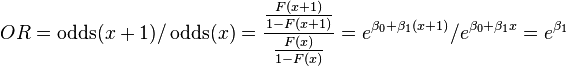
or for binary variable F(0) instead of F(x) and F(1) for F(x+1). This exponential relationship provides an interpretation for  : The odds multiply by
  for every 1-unit increase in x.[15]
Multiple explanatory variables
If there are multiple explanatory variables, the above expression  can be revised to
  Then when this is used in the equation relating the logged odds of a success to the values of the predictors, the linear regression will be a multiple regression with m explanators; the parameters
  for all j = 0, 1, 2, ..., m are all estimated.
Model fitting
Estimation
Because the model can be expressed as a generalized linear model (see below), for 0<p<1, ordinary least squares can suffice, with R-squared as the measure of goodness of fit in the fitting space. When p=0 or 1, more complex methods are required.
Maximum likelihood estimation
The regression coefficients are usually estimated using maximum likelihood estimation.[16] Unlike linear regression with normally distributed residuals, it is not possible to find a closed-form expression for the coefficient values that maximize the likelihood function, so that an iterative process must be used instead; for example Newton's method. This process begins with a tentative solution, revises it slightly to see if it can be improved, and repeats this revision until improvement is minute, at which point the process is said to have converged.[17]
In some instances the model may not reach convergence. Nonconvergence of a model indicates that the coefficients are not meaningful because the iterative process was unable to find appropriate solutions. A failure to converge may occur for a number of reasons: having a large ratio of predictors to cases, multicollinearity, sparseness, or complete separation.
- Having a large ratio of variables to cases results in an overly conservative Wald statistic (discussed below) and can lead to nonconvergence.
- Multicollinearity refers to unacceptably high correlations between predictors. As multicollinearity increases, coefficients remain unbiased but standard errors increase and the likelihood of model convergence decreases.[16] To detect multicollinearity amongst the predictors, one can conduct a linear regression analysis with the predictors of interest for the sole purpose of examining the tolerance statistic [16] used to assess whether multicollinearity is unacceptably high.
- Sparseness in the data refers to having a large proportion of empty cells (cells with zero counts). Zero cell counts are particularly problematic with categorical predictors. With continuous predictors, the model can infer values for the zero cell counts, but this is not the case with categorical predictors. The model will not converge with zero cell counts for categorical predictors because the natural logarithm of zero is an undefined value, so that final solutions to the model cannot be reached. To remedy this problem, researchers may collapse categories in a theoretically meaningful way or add a constant to all cells.[16]
- Another numerical problem that may lead to a lack of convergence is complete separation, which refers to the instance in which the predictors perfectly predict the criterion – all cases are accurately classified. In such instances, one should reexamine the data, as there is likely some kind of error.[14]
As a general rule of thumb, logistic regression models require a minimum of about 10 events per explaining variable (where event denotes the cases belonging to the less frequent category in the dependent variable).[18]
Minimum chi-squared estimator for grouped data
While individual data will have a dependent variable with a value of zero or one for every observation, with grouped data one observation is on a group of people who all share the same characteristics (e.g., demographic characteristics); in this case the researcher observes the proportion of people in the group for whom the response variable falls into one category or the other. If this proportion is neither zero nor one for any group, the minimum chi-squared estimator involves using weighted least squares to estimate a linear model in which the dependent variable is the logit of the proportion: that is, the log of the ratio of the fraction in one group to the fraction in the other group.[19]:pp.686–9
Evaluating goodness of fit
Goodness of fit in linear regression models is generally measured using the R2. Since this has no direct analog in logistic regression, various methods[19]:ch.21 including the following can be used instead.
Deviance and likelihood ratio tests
In linear regression analysis, one is concerned with partitioning variance via the sum of squares calculations – variance in the criterion is essentially divided into variance accounted for by the predictors and residual variance. In logistic regression analysis, deviance is used in lieu of sum of squares calculations.[20] Deviance is analogous to the sum of squares calculations in linear regression[14] and is a measure of the lack of fit to the data in a logistic regression model.[20] When a "saturated" model is available (a model with a theoretically perfect fit), deviance is calculated by comparing a given model with the saturated model.[14] This computation give the likelihood-ratio test:.[14]
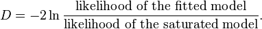
In the above equation D represents the deviance and ln represents the natural logarithm. The log of the likelihood ratio (the ratio of the fitted model to the saturated model) will produce a negative value, so the product is multiplied by negative two times its natural logarithm to produce a value with an approximate chi-squared distribution.[14] Smaller values indicate better fit as the fitted model deviates less from the saturated model. When assessed upon a chi-square distribution, nonsignificant chi-square values indicate very little unexplained variance and thus, good model fit. Conversely, a significant chi-square value indicates that a significant amount of the variance is unexplained.
When the saturated model is not available (a common case), deviance is calculated simply as (-2)x(log likelihood of the fitted model), and the reference to the saturated model's log likelihood can be removed from all that follows without harm.
Two measures of deviance are particularly important in logistic regression: null deviance and model deviance. The null deviance represents the difference between a model with only the intercept (which means "no predictors") and the saturated model. The model deviance represents the difference between a model with at least one predictor and the saturated model.[20] In this respect, the null model provides a baseline upon which to compare predictor models. Given that deviance is a measure of the difference between a given model and the saturated model, smaller values indicate better fit. Thus, to assess the contribution of a predictor or set of predictors, one can subtract the model deviance from the null deviance and assess the difference on a  chi-square distribution with degrees of freedom[14] equal to the difference in the number of parameters estimated.
Let


Then
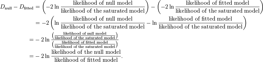
If the model deviance is significantly smaller than the null deviance then one can conclude that the predictor or set of predictors significantly improved model fit. This is analogous to the F-test used in linear regression analysis to assess the significance of prediction.[20]
Pseudo-R2s
In linear regression the squared multiple correlation, R2 is used to assess goodness of fit as it represents the proportion of variance in the criterion that is explained by the predictors.[20] In logistic regression analysis, there is no agreed upon analogous measure, but there are several competing measures each with limitations.[20] Three of the most commonly used indices are examined on this page beginning with the likelihood ratio R2, R2L:[20]
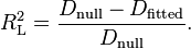
This is the most analogous index to the squared multiple correlation in linear regression.[16] It represents the proportional reduction in the deviance wherein the deviance is treated as a measure of variation analogous but not identical to the variance in linear regression analysis.[16] One limitation of the likelihood ratio R2 is that it is not monotonically related to the odds ratio,[20] meaning that it does not necessarily increase as the odds ratio increases and does not necessarily decrease as the odds ratio decreases.
The Cox and Snell R2 is an alternative index of goodness of fit related to the R2 value from linear regression. The Cox and Snell index is problematic as its maximum value is .75, when the variance is at its maximum (.25). The Nagelkerke R2 provides a correction to the Cox and Snell R2 so that the maximum value is equal to one. Nevertheless, the Cox and Snell and likelihood ratio R2s show greater agreement with each other than either does with the Nagelkerke R2.[20] Of course, this might not be the case for values exceeding .75 as the Cox and Snell index is capped at this value. The likelihood ratio R2 is often preferred to the alternatives as it is most analogous to R2 in linear regression, is independent of the base rate (both Cox and Snell and Nagelkerke R2s increase as the proportion of cases increase from 0 to .5) and varies between 0 and 1.
A word of caution is in order when interpreting pseudo-R2 statistics. The reason these indices of fit are referred to as pseudo R2 is that they do not represent the proportionate reduction in error as the R2 in linear regression does.[20] Linear regression assumes homoscedasticity, that the error variance is the same for all values of the criterion. Logistic regression will always be heteroscedastic – the error variances differ for each value of the predicted score. For each value of the predicted score there would be a different value of the proportionate reduction in error. Therefore, it is inappropriate to think of R2 as a proportionate reduction in error in a universal sense in logistic regression.[20]
Hosmer–Lemeshow test
The Hosmer–Lemeshow test uses a test statistic that asymptotically follows a  distribution to assess whether or not the observed event rates match expected event rates in subgroups of the model population.
Evaluating binary classification performance
If the estimated probabilities are to be used to classify each observation of independent variable values as predicting the category that the dependent variable is found in, the various methods below for judging the model's suitability in out-of-sample forecasting can also be used on the data that were used for estimation—accuracy, precision (also called positive predictive value), recall (also called sensitivity), specificity and negative predictive value. In each of these evaluative methods, an aspect of the model's effectiveness in assigning instances to the correct categories is measured.
Coefficients
After fitting the model, it is likely that researchers will want to examine the contribution of individual predictors. To do so, they will want to examine the regression coefficients. In linear regression, the regression coefficients represent the change in the criterion for each unit change in the predictor.[20] In logistic regression, however, the regression coefficients represent the change in the logit for each unit change in the predictor. Given that the logit is not intuitive, researchers are likely to focus on a predictor's effect on the exponential function of the regression coefficient – the odds ratio (see definition). In linear regression, the significance of a regression coefficient is assessed by computing a t test. In logistic regression, there are several different tests designed to assess the significance of an individual predictor, most notably the likelihood ratio test and the Wald statistic.
Likelihood ratio test
The likelihood-ratio test discussed above to assess model fit is also the recommended procedure to assess the contribution of individual "predictors" to a given model.[14][16][20] In the case of a single predictor model, one simply compares the deviance of the predictor model with that of the null model on a chi-square distribution with a single degree of freedom. If the predictor model has a significantly smaller deviance (c.f chi-square using the difference in degrees of freedom of the two models), then one can conclude that there is a significant association between the "predictor" and the outcome. Although some common statistical packages (e.g. SPSS) do provide likelihood ratio test statistics, without this computationally intensive test it would be more difficult to assess the contribution of individual predictors in the multiple logistic regression case. To assess the contribution of individual predictors one can enter the predictors hierarchically, comparing each new model with the previous to determine the contribution of each predictor.[20] There is some debate among statisticians about the appropriateness of so-called "stepwise" procedures. The fear is that they may not preserve nominal statistical properties and may become misleading.
Wald statistic
Alternatively, when assessing the contribution of individual predictors in a given model, one may examine the significance of the Wald statistic. The Wald statistic, analogous to the t-test in linear regression, is used to assess the significance of coefficients. The Wald statistic is the ratio of the square of the regression coefficient to the square of the standard error of the coefficient and is asymptotically distributed as a chi-square distribution.[16]

Although several statistical packages (e.g., SPSS, SAS) report the Wald statistic to assess the contribution of individual predictors, the Wald statistic has limitations. When the regression coefficient is large, the standard error of the regression coefficient also tends to be large increasing the probability of Type-II error. The Wald statistic also tends to be biased when data are sparse.[20]
Case-control sampling
Suppose cases are rare. Then we might wish to sample them more frequently than their prevalence in the population. For example, suppose there is a disease that affects 1 person in 10,000 and to collect our data we need to do a complete physical. It may be too expensive to do thousands of physicals of healthy people in order to obtain data for only a few diseased individuals. Thus, we may evaluate more diseased individuals. This is also called unbalanced data. As a rule of thumb, sampling controls at a rate of five times the number of cases will produce sufficient control data.[21]
If we form a logistic model from such data, if the model is correct, the parameters are all correct except for . We can correct if we know the true prevalence as follows:[21]
where  is the true prevalence and
  is the prevalence in the sample.
Formal mathematical specification
There are various equivalent specifications of logistic regression, which fit into different types of more general models. These different specifications allow for different sorts of useful generalizations.
Setup
The basic setup of logistic regression is the same as for standard linear regression.
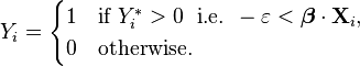
It is assumed that we have a series of N observed data points. Each data point i consists of a set of m explanatory variables x1,i ... xm,i (also called independent variables, predictor variables, input variables, features, or attributes), and an associated binary-valued outcome variable Yi (also known as a dependent variable, response variable, output variable, outcome variable or class variable), i.e. it can assume only the two possible values 0 (often meaning "no" or "failure") or 1 (often meaning "yes" or "success"). The goal of logistic regression is to explain the relationship between the explanatory variables and the outcome, so that an outcome can be predicted for a new set of explanatory variables.
Some examples:
- The observed outcomes are the presence or absence of a given disease (e.g. diabetes) in a set of patients, and the explanatory variables might be characteristics of the patients thought to be pertinent (sex, race, age, blood pressure, body-mass index, etc.).
- The observed outcomes are the votes (e.g. Democratic or Republican) of a set of people in an election, and the explanatory variables are the demographic characteristics of each person (e.g. sex, race, age, income, etc.). In such a case, one of the two outcomes is arbitrarily coded as 1, and the other as 0.
As in linear regression, the outcome variables Yi are assumed to depend on the explanatory variables x1,i ... xm,i.
- Explanatory variables
As shown above in the above examples, the explanatory variables may be of any type: real-valued, binary, categorical, etc. The main distinction is between continuous variables (such as income, age and blood pressure) and discrete variables (such as sex or race). Discrete variables referring to more than two possible choices are typically coded using dummy variables (or indicator variables), that is, separate explanatory variables taking the value 0 or 1 are created for each possible value of the discrete variable, with a 1 meaning "variable does have the given value" and a 0 meaning "variable does not have that value". For example, a four-way discrete variable of blood type with the possible values "A, B, AB, O" can be converted to four separate two-way dummy variables, "is-A, is-B, is-AB, is-O", where only one of them has the value 1 and all the rest have the value 0. This allows for separate regression coefficients to be matched for each possible value of the discrete variable. (In a case like this, only three of the four dummy variables are independent of each other, in the sense that once the values of three of the variables are known, the fourth is automatically determined. Thus, it is necessary to encode only three of the four possibilities as dummy variables. This also means that when all four possibilities are encoded, the overall model is not identifiable in the absence of additional constraints such as a regularization constraint. Theoretically, this could cause problems, but in reality almost all logistic regression models are fitted with regularization constraints.)
- Outcome variables
Formally, the outcomes Yi are described as being Bernoulli-distributed data, where each outcome is determined by an unobserved probability pi that is specific to the outcome at hand, but related to the explanatory variables. This can be expressed in any of the following equivalent forms:
![\begin{align}
Y_i\mid x_{1,i},\ldots,x_{m,i} \ & \sim \operatorname{Bernoulli}(p_i) \\
\mathbb{E}[Y_i\mid x_{1,i},\ldots,x_{m,i}] &= p_i \\
\Pr(Y_i=y_i\mid x_{1,i},\ldots,x_{m,i}) &=
\begin{cases}
p_i & \text{if }y_i=1 \\
1-p_i & \text{if }y_i=0
\end{cases}
\\
\Pr(Y_i=y_i\mid x_{1,i},\ldots,x_{m,i}) &= p_i^{y_i} (1-p_i)^{(1-y_i)}
\end{align}](../I/m/b68112dbf60d6444d8418a46c77ea731.png)
The meanings of these four lines are:
- The first line expresses the probability distribution of each Yi: Conditioned on the explanatory variables, it follows a Bernoulli distribution with parameters pi, the probability of the outcome of 1 for trial i. As noted above, each separate trial has its own probability of success, just as each trial has its own explanatory variables. The probability of success pi is not observed, only the outcome of an individual Bernoulli trial using that probability.
- The second line expresses the fact that the expected value of each Yi is equal to the probability of success pi, which is a general property of the Bernoulli distribution. In other words, if we run a large number of Bernoulli trials using the same probability of success pi, then take the average of all the 1 and 0 outcomes, then the result would be close to pi. This is because doing an average this way simply computes the proportion of successes seen, which we expect to converge to the underlying probability of success.
- The third line writes out the probability mass function of the Bernoulli distribution, specifying the probability of seeing each of the two possible outcomes.
- The fourth line is another way of writing the probability mass function, which avoids having to write separate cases and is more convenient for certain types of calculations. This relies on the fact that Yi can take only the value 0 or 1. In each case, one of the exponents will be 1, "choosing" the value under it, while the other is 0, "canceling out" the value under it. Hence, the outcome is either pi or 1 − pi, as in the previous line.
- Linear predictor function
The basic idea of logistic regression is to use the mechanism already developed for linear regression by modeling the probability pi using a linear predictor function, i.e. a linear combination of the explanatory variables and a set of regression coefficients that are specific to the model at hand but the same for all trials. The linear predictor function  for a particular data point i is written as:

where  are regression coefficients indicating the relative effect of a particular explanatory variable on the outcome.
The model is usually put into a more compact form as follows:
- The regression coefficients β0, β1, ..., βm are grouped into a single vector β of size m + 1.
- For each data point i, an additional explanatory pseudo-variable x0,i is added, with a fixed value of 1, corresponding to the intercept coefficient β0.
- The resulting explanatory variables x0,i, x1,i, ..., xm,i are then grouped into a single vector Xi of size m + 1.
This makes it possible to write the linear predictor function as follows:

using the notation for a dot product between two vectors.
As a generalized linear model
The particular model used by logistic regression, which distinguishes it from standard linear regression and from other types of regression analysis used for binary-valued outcomes, is the way the probability of a particular outcome is linked to the linear predictor function:
![\operatorname{logit}(\mathbb{E}[Y_i\mid x_{1,i},\ldots,x_{m,i}]) = \operatorname{logit}(p_i)=\ln\left(\frac{p_i}{1-p_i}\right) = \beta_0 + \beta_1 x_{1,i} + \cdots + \beta_m x_{m,i}](../I/m/7010ce2c8df19e884f2fb3a75cc9bee2.png)
Written using the more compact notation described above, this is:
![\operatorname{logit}(\mathbb{E}[Y_i\mid \mathbf{X}_i]) = \operatorname{logit}(p_i)=\ln\left(\frac{p_i}{1-p_i}\right) = \boldsymbol\beta \cdot \mathbf{X}_i](../I/m/37dc6b8bfa450a83f545a36b98cbc2f2.png)
This formulation expresses logistic regression as a type of generalized linear model, which predicts variables with various types of probability distributions by fitting a linear predictor function of the above form to some sort of arbitrary transformation of the expected value of the variable.
The intuition for transforming using the logit function (the natural log of the odds) was explained above. It also has the practical effect of converting the probability (which is bounded to be between 0 and 1) to a variable that ranges over  — thereby matching the potential range of the linear prediction function on the right side of the equation.
Note that both the probabilities pi and the regression coefficients are unobserved, and the means of determining them is not part of the model itself. They are typically determined by some sort of optimization procedure, e.g. maximum likelihood estimation, that finds values that best fit the observed data (i.e. that give the most accurate predictions for the data already observed), usually subject to regularization conditions that seek to exclude unlikely values, e.g. extremely large values for any of the regression coefficients. The use of a regularization condition is equivalent to doing maximum a posteriori (MAP) estimation, an extension of maximum likelihood. (Regularization is most commonly done using a squared regularizing function, which is equivalent to placing a zero-mean Gaussian prior distribution on the coefficients, but other regularizers are also possible.) Whether or not regularization is used, it is usually not possible to find a closed-form solution; instead, an iterative numerical method must be used, such as iteratively reweighted least squares (IRLS) or, more commonly these days, a quasi-Newton method such as the L-BFGS method.
The interpretation of the βj parameter estimates is as the additive effect on the log of the odds for a unit change in the jth explanatory variable. In the case of a dichotomous explanatory variable, for instance gender,  is the estimate of the odds of having the outcome for, say, males compared with females.
An equivalent formula uses the inverse of the logit function, which is the logistic function, i.e.:
![\mathbb{E}[Y_i\mid \mathbf{X}_i] = p_i = \operatorname{logit}^{-1}(\boldsymbol\beta \cdot \mathbf{X}_i) = \frac{1}{1+e^{-\boldsymbol\beta \cdot \mathbf{X}_i}}](../I/m/48a81d42f025615151125f49cdce007a.png)
The formula can also be written (somewhat awkwardly) as a probability distribution (specifically, using a probability mass function):

As a latent-variable model
The above model has an equivalent formulation as a latent-variable model. This formulation is common in the theory of discrete choice models, and makes it easier to extend to certain more complicated models with multiple, correlated choices, as well as to compare logistic regression to the closely related probit model.
Imagine that, for each trial i, there is a continuous latent variable Yi* (i.e. an unobserved random variable) that is distributed as follows:

where

i.e. the latent variable can be written directly in terms of the linear predictor function and an additive random error variable that is distributed according to a standard logistic distribution.
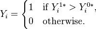
Then Yi can be viewed as an indicator for whether this latent variable is positive:
The choice of modeling the error variable specifically with a standard logistic distribution, rather than a general logistic distribution with the location and scale set to arbitrary values, seems restrictive, but in fact it is not. It must be kept in mind that we can choose the regression coefficients ourselves, and very often can use them to offset changes in the parameters of the error variable's distribution. For example, a logistic error-variable distribution with a non-zero location parameter μ (which sets the mean) is equivalent to a distribution with a zero location parameter, where μ has been added to the intercept coefficient. Both situations produce the same value for Yi* regardless of settings of explanatory variables. Similarly, an arbitrary scale parameter s is equivalent to setting the scale parameter to 1 and then dividing all regression coefficients by s. In the latter case, the resulting value of Yi* will be smaller by a factor of s than in the former case, for all sets of explanatory variables — but critically, it will always remain on the same side of 0, and hence lead to the same Yi choice.
(Note that this predicts that the irrelevancy of the scale parameter may not carry over into more complex models where more than two choices are available.)
It turns out that this formulation is exactly equivalent to the preceding one, phrased in terms of the generalized linear model and without any latent variables. This can be shown as follows, using the fact that the cumulative distribution function (CDF) of the standard logistic distribution is the logistic function, which is the inverse of the logit function, i.e.

Then:

This formulation—which is standard in discrete choice models—makes clear the relationship between logistic regression (the "logit model") and the probit model, which uses an error variable distributed according to a standard normal distribution instead of a standard logistic distribution. Both the logistic and normal distributions are symmetric with a basic unimodal, "bell curve" shape. The only difference is that the logistic distribution has somewhat heavier tails, which means that it is less sensitive to outlying data (and hence somewhat more robust to model mis-specifications or erroneous data).
As a two-way latent-variable model
Yet another formulation uses two separate latent variables:
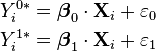
where
where EV1(0,1) is a standard type-1 extreme value distribution: i.e.

Then
This model has a separate latent variable and a separate set of regression coefficients for each possible outcome of the dependent variable. The reason for this separation is that it makes it easy to extend logistic regression to multi-outcome categorical variables, as in the multinomial logit model. In such a model, it is natural to model each possible outcome using a different set of regression coefficients. It is also possible to motivate each of the separate latent variables as the theoretical utility associated with making the associated choice, and thus motivate logistic regression in terms of utility theory. (In terms of utility theory, a rational actor always chooses the choice with the greatest associated utility.) This is the approach taken by economists when formulating discrete choice models, because it both provides a theoretically strong foundation and facilitates intuitions about the model, which in turn makes it easy to consider various sorts of extensions. (See the example below.)
The choice of the type-1 extreme value distribution seems fairly arbitrary, but it makes the mathematics work out, and it may be possible to justify its use through rational choice theory.
It turns out that this model is equivalent to the previous model, although this seems non-obvious, since there are now two sets of regression coefficients and error variables, and the error variables have a different distribution. In fact, this model reduces directly to the previous one with the following substitutions:

An intuition for this comes from the fact that, since we choose based on the maximum of two values, only their difference matters, not the exact values — and this effectively removes one degree of freedom. Another critical fact is that the difference of two type-1 extreme-value-distributed variables is a logistic distribution, i.e. if 
We can demonstrate the equivalent as follows:
![\begin{align}
& \Pr(Y_i=1\mid\mathbf{X}_i) \\[4pt]
= {} & \Pr(Y_i^{1\ast} > Y_i^{0\ast}\mid\mathbf{X}_i) & \\
= {} & \Pr(Y_i^{1\ast} - Y_i^{0\ast} > 0\mid\mathbf{X}_i) & \\
= {} & \Pr(\boldsymbol\beta_1 \cdot \mathbf{X}_i + \varepsilon_1 - (\boldsymbol\beta_0 \cdot \mathbf{X}_i + \varepsilon_0) > 0) & \\
= {} & \Pr((\boldsymbol\beta_1 \cdot \mathbf{X}_i - \boldsymbol\beta_0 \cdot \mathbf{X}_i) + (\varepsilon_1 - \varepsilon_0) > 0) & \\
= {} & \Pr((\boldsymbol\beta_1 - \boldsymbol\beta_0) \cdot \mathbf{X}_i + (\varepsilon_1 - \varepsilon_0) > 0) & \\
= {} & \Pr((\boldsymbol\beta_1 - \boldsymbol\beta_0) \cdot \mathbf{X}_i + \varepsilon > 0) & & \text{(substitute }\varepsilon\text{ as above)} \\
= {} & \Pr(\boldsymbol\beta \cdot \mathbf{X}_i + \varepsilon > 0) & & \text{(substitute }\boldsymbol\beta\text{ as above)} \\
= {} & \Pr(\varepsilon > -\boldsymbol\beta \cdot \mathbf{X}_i) & & \text{(now, same as above model)}\\
= {} & \Pr(\varepsilon < \boldsymbol\beta \cdot \mathbf{X}_i) & \\
= {} & \operatorname{logit}^{-1}(\boldsymbol\beta \cdot \mathbf{X}_i) & \\
= {} & p_i
\end{align}](../I/m/9973338ac6cde0f94ec39756c5cb148e.png)
Example
As an example, consider a province-level election where the choice is between a right-of-center party, a left-of-center party, and a secessionist party (e.g. the Parti Québécois, which wants Quebec to secede from Canada). We would then use three latent variables, one for each choice. Then, in accordance with utility theory, we can then interpret the latent variables as expressing the utility that results from making each of the choices. We can also interpret the regression coefficients as indicating the strength that the associated factor (i.e. explanatory variable) has in contributing to the utility — or more correctly, the amount by which a unit change in an explanatory variable changes the utility of a given choice. A voter might expect that the right-of-center party would lower taxes, especially on rich people. This would give low-income people no benefit, i.e. no change in utility (since they usually don't pay taxes); would cause moderate benefit (i.e. somewhat more money, or moderate utility increase) for middle-incoming people; and would cause significant benefits for high-income people. On the other hand, the left-of-center party might be expected to raise taxes and offset it with increased welfare and other assistance for the lower and middle classes. This would cause significant positive benefit to low-income people, perhaps weak benefit to middle-income people, and significant negative benefit to high-income people. Finally, the secessionist party would take no direct actions on the economy, but simply secede. A low-income or middle-income voter might expect basically no clear utility gain or loss from this, but a high-income voter might expect negative utility, since he/she is likely to own companies, which will have a harder time doing business in such an environment and probably lose money.
These intuitions can be expressed as follows:
| Center-right | Center-left | Secessionist | |
|---|---|---|---|
| High-income | strong + | strong − | strong − |
| Middle-income | moderate + | weak + | none |
| Low-income | none | strong + | none |
This clearly shows that
- Separate sets of regression coefficients need to exist for each choice. When phrased in terms of utility, this can be seen very easily. Different choices have different effects on net utility; furthermore, the effects vary in complex ways that depend on the characteristics of each individual, so there need to be separate sets of coefficients for each characteristic, not simply a single extra per-choice characteristic.
- Even though income is a continuous variable, its effect on utility is too complex for it to be treated as a single variable. Either it needs to be directly split up into ranges, or higher powers of income need to be added so that polynomial regression on income is effectively done.
As a "log-linear" model
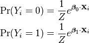
Yet another formulation combines the two-way latent variable formulation above with the original formulation higher up without latent variables, and in the process provides a link to one of the standard formulations of the multinomial logit.
Here, instead of writing the logit of the probabilities pi as a linear predictor, we separate the linear predictor into two, one for each of the two outcomes:

Note that two separate sets of regression coefficients have been introduced, just as in the two-way latent variable model, and the two equations appear a form that writes the logarithm of the associated probability as a linear predictor, with an extra term  at the end. This term, as it turns out, serves as the normalizing factor ensuring that the result is a distribution. This can be seen by exponentiating both sides:
In this form it is clear that the purpose of Z is to ensure that the resulting distribution over Yi is in fact a probability distribution, i.e. it sums to 1. This means that Z is simply the sum of all un-normalized probabilities, and by dividing each probability by Z, the probabilities become "normalized". That is:

and the resulting equations are
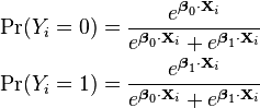
Or generally:

This shows clearly how to generalize this formulation to more than two outcomes, as in multinomial logit. Note that this general formulation is exactly the Softmax function as in

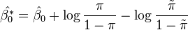
In order to prove that this is equivalent to the previous model, note that the above model is overspecified, in that  and
and  cannot be independently specified: rather
  so knowing one automatically determines the other. As a result, the model is nonidentifiable, in that multiple combinations of β0 and β1 will produce the same probabilities for all possible explanatory variables. In fact, it can be seen that adding any constant vector to both of them will produce the same probabilities:

As a result, we can simplify matters, and restore identifiability, by picking an arbitrary value for one of the two vectors. We choose to set  Then,
Then,
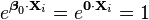
and so
which shows that this formulation is indeed equivalent to the previous formulation. (As in the two-way latent variable formulation, any settings where  will produce equivalent results.)
Note that most treatments of the multinomial logit model start out either by extending the "log-linear" formulation presented here or the two-way latent variable formulation presented above, since both clearly show the way that the model could be extended to multi-way outcomes. In general, the presentation with latent variables is more common in econometrics and political science, where discrete choice models and utility theory reign, while the "log-linear" formulation here is more common in computer science, e.g. machine learning and natural language processing.
As a single-layer perceptron
The model has an equivalent formulation

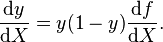
This functional form is commonly called a single-layer perceptron or single-layer artificial neural network. A single-layer neural network computes a continuous output instead of a step function. The derivative of pi with respect to X = (x1, ..., xk) is computed from the general form:

where f(X) is an analytic function in X. With this choice, the single-layer neural network is identical to the logistic regression model. This function has a continuous derivative, which allows it to be used in backpropagation. This function is also preferred because its derivative is easily calculated:
In terms of binomial data
A closely related model assumes that each i is associated not with a single Bernoulli trial but with ni independent identically distributed trials, where the observation Yi is the number of successes observed (the sum of the individual Bernoulli-distributed random variables), and hence follows a binomial distribution:

An example of this distribution is the fraction of seeds (pi) that germinate after ni are planted.
In terms of expected values, this model is expressed as follows:
![p_i = \mathbb{E}\left[\left.\frac{Y_i}{n_{i}}\,\right|\,\mathbf{X}_i \right],](../I/m/e91633f859f0a2a245324fc373894b94.png)
so that
![\operatorname{logit}\left(\mathbb{E}\left[\left.\frac{Y_i}{n_{i}}\,\right|\,\mathbf{X}_i \right]\right) = \operatorname{logit}(p_i)=\ln\left(\frac{p_i}{1-p_i}\right) = \boldsymbol\beta \cdot \mathbf{X}_i,](../I/m/0250d3e9f9d0344c6718cf1f46f29deb.png)
Or equivalently:

This model can be fit using the same sorts of methods as the above more basic model.
Bayesian logistic regression

 vs.
vs.  , which makes the slopes the same at the origin. This shows the heavier tails of the logistic distribution.
In a Bayesian statistics context, prior distributions are normally placed on the regression coefficients, usually in the form of Gaussian distributions. Unfortunately, the Gaussian distribution is not the conjugate prior of the likelihood function in logistic regression. As a result, the posterior distribution is difficult to calculate, even using standard simulation algorithms (e.g. Gibbs sampling).
There are various possibilities:
- Don't do a proper Bayesian analysis, but simply compute a maximum a posteriori point estimate of the parameters. This is common, for example, in "maximum entropy" classifiers in machine learning.
- Use a more general approximation method such as the Metropolis–Hastings algorithm.
- Draw a Markov chain Monte Carlo sample from the exact posterior by using the Independent Metropolis–Hastings algorithm with heavy-tailed multivariate candidate distribution found by matching the mode and curvature at the mode of the normal approximation to the posterior and then using the Student’s t shape with low degrees of freedom.[22] This is shown to have excellent convergence properties.
- Use a latent variable model and approximate the logistic distribution using a more tractable distribution, e.g. a Student's t-distribution or a mixture of normal distributions.
- Do probit regression instead of logistic regression. This is actually a special case of the previous situation, using a normal distribution in place of a Student's t, mixture of normals, etc. This will be less accurate but has the advantage that probit regression is extremely common, and a ready-made Bayesian implementation may already be available.
- Use the Laplace approximation of the posterior distribution.[23] This approximates the posterior with a Gaussian distribution. This is not a terribly good approximation, but it suffices if all that is desired is an estimate of the posterior mean and variance. In such a case, an approximation scheme such as variational Bayes can be used.[24]
Gibbs sampling with an approximating distribution
As shown above, logistic regression is equivalent to a latent variable model with an error variable distributed according to a standard logistic distribution. The overall distribution of the latent variable  is also a logistic distribution, with the mean equal to
  (i.e. the fixed quantity added to the error variable). This model considerably simplifies the application of techniques such as Gibbs sampling. However, sampling the regression coefficients is still difficult, because of the lack of conjugacy between the normal and logistic distributions. Changing the prior distribution over the regression coefficients is of no help, because the logistic distribution is not in the exponential family and thus has no conjugate prior.
One possibility is to use a more general Markov chain Monte Carlo technique, such as the Metropolis–Hastings algorithm, which can sample arbitrary distributions. Another possibility, however, is to replace the logistic distribution with a similar-shaped distribution that is easier to work with using Gibbs sampling. In fact, the logistic and normal distributions have a similar shape, and thus one possibility is simply to have normally distributed errors. Because the normal distribution is conjugate to itself, sampling the regression coefficients becomes easy. In fact, this model is exactly the model used in probit regression.
However, the normal and logistic distributions differ in that the logistic has heavier tails. As a result, it is more robust to inaccuracies in the underlying model (which are inevitable, in that the model is essentially always an approximation) or to errors in the data. Probit regression loses some of this robustness.
Another alternative is to use errors distributed as a Student's t-distribution. The Student's t-distribution has heavy tails, and is easy to sample from because it is the compound distribution of a normal distribution with variance distributed as an inverse gamma distribution. In other words, if a normal distribution is used for the error variable, and another latent variable, following an inverse gamma distribution, is added corresponding to the variance of this error variable, the marginal distribution of the error variable will follow a Student's t distribution. Because of the various conjugacy relationships, all variables in this model are easy to sample from.
The Student's t distribution that best approximates a standard logistic distribution can be determined by matching the moments of the two distributions. The Student's t distribution has three parameters, and since the skewness of both distributions is always 0, the first four moments can all be matched, using the following equations:
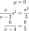
This yields the following values:
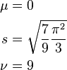
The following graphs compare the standard logistic distribution with the Student's t distribution that matches the first four moments using the above-determined values, as well as the normal distribution that matches the first two moments. Note how much closer the Student's t distribution agrees, especially in the tails. Beyond about two standard deviations from the mean, the logistic and normal distributions diverge rapidly, but the logistic and Student's t distributions don't start diverging significantly until more than 5 standard deviations away.
(Another possibility, also amenable to Gibbs sampling, is to approximate the logistic distribution using a mixture density of normal distributions.)
 Comparison of logistic and approximating distributions (t, normal). |
 Tails of distributions. |
 Further tails of distributions. |
 Extreme tails of distributions. |
Extensions
There are large numbers of extensions:
- Multinomial logistic regression (or multinomial logit) handles the case of a multi-way categorical dependent variable (with unordered values, also called "classification"). Note that the general case of having dependent variables with more than two values is termed polytomous regression.
- Ordered logistic regression (or ordered logit) handles ordinal dependent variables (ordered values).
- Mixed logit is an extension of multinomial logit that allows for correlations among the choices of the dependent variable.
- An extension of the logistic model to sets of interdependent variables is the conditional random field.
Model suitability
A way to measure a model's suitability is to assess the model against a set of data that was not used to create the model.[25] The class of techniques is called cross-validation. This holdout model assessment method is particularly valuable when data are collected in different settings (e.g., at different times or places) or when models are assumed to be generalizable.
To measure the suitability of a binary regression model, one can classify both the actual value and the predicted value of each observation as either 0 or 1.[26] The predicted value of an observation can be set equal to 1 if the estimated probability that the observation equals 1 is above  , and set equal to 0 if the estimated probability is below . Here logistic regression is being used as a binary classification model. There are four possible combined classifications:
- prediction of 0 when the holdout sample has a 0 (True Negatives, the number of which is TN)
- prediction of 0 when the holdout sample has a 1 (False Negatives, the number of which is FN)
- prediction of 1 when the holdout sample has a 0 (False Positives, the number of which is FP)
- prediction of 1 when the holdout sample has a 1 (True Positives, the number of which is TP)
These classifications are used to calculate accuracy, precision (also called positive predictive value), recall (also called sensitivity), specificity and negative predictive value:
-
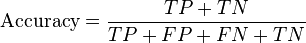 = fraction of observations with correct predicted classification
-
 = Fraction of predicted positives that are correct
 = fraction of predicted negatives that are correct
-
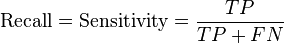 = fraction of observations that are actually 1 with a correct predicted classification
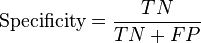 = fraction of observations that are actually 0 with a correct predicted classification
See also
- Logistic function
- Discrete choice
- Jarrow–Turnbull model
- Limited dependent variable
- Multinomial logit model
- Ordered logit
- Hosmer–Lemeshow test
- Brier score
- MLPACK - contains a C++ implementation of logistic regression
References
- ↑ 1.0 1.1 1.2 David A. Freedman (2009). Statistical Models: Theory and Practice. Cambridge University Press. p. 128.
- ↑ Cox, DR (1958). "The regression analysis of binary sequences (with discussion)". J Roy Stat Soc B 20: 215–242.
- ↑ 3.0 3.1 Walker, SH; Duncan, DB (1967). "Estimation of the probability of an event as a function of several independent variables". Biometrika 54: 167–178.
- ↑ Gareth James; Daniela Witten; Trevor Hastie; Robert Tibshirani (2013). An Introduction to Statistical Learning. Springer. p. 6.
- ↑ Boyd, C. R.; Tolson, M. A.; Copes, W. S. (1987). "Evaluating trauma care: The TRISS method. Trauma Score and the Injury Severity Score". The Journal of trauma 27 (4): 370–378. doi:10.1097/00005373-198704000-00005. PMID 3106646.
- ↑ Kologlu M., Elker D., Altun H., Sayek I. Valdation of MPI and OIA II in two different groups of patients with secondary peritonitis // Hepato-Gastroenterology. – 2001. – Vol. 48, № 37. – P. 147-151.
- ↑ Biondo S., Ramos E., Deiros M. et al. Prognostic factors for mortality in left colonic peritonitis: a new scoring system // J. Am. Coll. Surg. – 2000. – Vol. 191, № 6. – Р. 635-642.
- ↑ Marshall J.C., Cook D.J., Christou N.V. et al. Multiple Organ Dysfunction Score: A reliable descriptor of a complex clinical outcome // Crit. Care Med. – 1995. – Vol. 23. – P. 1638-1652.
- ↑ Le Gall J.-R., Lemeshow S., Saulnier F. A new Simplified Acute Physiology Score (SAPS II) based on a European/North American multicenter study // JAMA. – 1993. – Vol. 270. – P. 2957-2963.
- ↑ Truett, J; Cornfield, J; Kannel, W (1967). "A multivariate analysis of the risk of coronary heart disease in Framingham". Journal of chronic diseases 20 (7): 511–24. PMID 6028270.
- ↑ Harrell, Frank E. (2001). Regression Modeling Strategies. Springer-Verlag. ISBN 0-387-95232-2.
- ↑ M. Strano; B.M. Colosimo (2006). "Logistic regression analysis for experimental determination of forming limit diagrams". International Journal of Machine Tools and Manufacture 46 (6). doi:10.1016/j.ijmachtools.2005.07.005.
- ↑ Palei, S. K.; Das, S. K. (2009). "Logistic regression model for prediction of roof fall risks in bord and pillar workings in coal mines: An approach". Safety Science 47: 88. doi:10.1016/j.ssci.2008.01.002.
- ↑ 14.0 14.1 14.2 14.3 14.4 14.5 14.6 14.7 14.8 14.9 14.10 Hosmer, David W.; Lemeshow, Stanley (2000). Applied Logistic Regression (2nd ed.). Wiley. ISBN 0-471-35632-8.
- ↑ http://www.planta.cn/forum/files_planta/introduction_to_categorical_data_analysis_805.pdf
- ↑ 16.0 16.1 16.2 16.3 16.4 16.5 16.6 16.7 Menard, Scott W. (2002). Applied Logistic Regression (2nd ed.). SAGE. ISBN 978-0-7619-2208-7.
- ↑ Menard ch 1.3
- ↑ Peduzzi, P; Concato, J; Kemper, E; Holford, TR; Feinstein, AR (December 1996). "A simulation study of the number of events per variable in logistic regression analysis.". Journal of Clinical Epidemiology 49 (12): 1373–9. doi:10.1016/s0895-4356(96)00236-3. PMID 8970487.
- ↑ 19.0 19.1 Greene, William N. (2003). Econometric Analysis (Fifth ed.). Prentice-Hall. ISBN 0-13-066189-9.
- ↑ 20.0 20.1 20.2 20.3 20.4 20.5 20.6 20.7 20.8 20.9 20.10 20.11 20.12 20.13 20.14 Cohen, Jacob; Cohen, Patricia; West, Steven G.; Aiken, Leona S. (2002). Applied Multiple Regression/Correlation Analysis for the Behavioral Sciences (3rd ed.). Routledge. ISBN 978-0-8058-2223-6.
- ↑ 21.0 21.1 https://class.stanford.edu/c4x/HumanitiesScience/StatLearning/asset/classification.pdf slide 16
- ↑ Bolstad, William M. (2010). Understandeing Computational Bayesian Statistics. Wiley. ISBN 978-0-470-04609-8.
- ↑ Bishop, Christopher M. "Chapter 4. Linear Models for Classification". Pattern Recognition and Machine Learning. Springer Science+Business Media, LLC. pp. 217–218. ISBN 978-0387-31073-2.
- ↑ Bishop, Christopher M. "Chapter 10. Approximate Inference". Pattern Recognition and Machine Learning. Springer Science+Business Media, LLC. pp. 498–505. ISBN 978-0387-31073-2.
- ↑ Jonathan Mark and Michael A. Goldberg (2001). Multiple Regression Analysis and Mass Assessment: A Review of the Issues. The Appraisal Journal, Jan. pp. 89–109
- ↑ Myers, J. H.; Forgy, E. W. (1963). "The Development of Numerical Credit Evaluation Systems". J. Amer. Statist. Assoc. 58 (303): 799–806. doi:10.1080/01621459.1963.10500889.
Further reading
- Agresti, Alan. (2002). Categorical Data Analysis. New York: Wiley-Interscience. ISBN 0-471-36093-7.
- Amemiya, T. (1985). Advanced Econometrics. Harvard University Press. ISBN 0-674-00560-0.
- Balakrishnan, N. (1991). Handbook of the Logistic Distribution. Marcel Dekker, Inc. ISBN 978-0-8247-8587-1.
- Greene, William H. (2003). Econometric Analysis, fifth edition. Prentice Hall. ISBN 0-13-066189-9.
- Hilbe, Joseph M. (2009). Logistic Regression Models. Chapman & Hall/CRC Press. ISBN 978-1-4200-7575-5.
- Howell, David C. (2010). Statistical Methods for Psychology, 7th ed. Belmont, CA; Thomson Wadsworth. ISBN 978-0-495-59786-5.
- Peduzzi, P.; J. Concato, E. Kemper, T.R. Holford, A.R. Feinstein (1996). "A simulation study of the number of events per variable in logistic regression analysis". Journal of Clinical Epidemiology 49 (12): 1373–1379. doi:10.1016/s0895-4356(96)00236-3. PMID 8970487.
External links
| Wikiversity has learning materials about Logistic regression |
- Econometrics Lecture (topic: Logit model) on YouTube by Mark Thoma
- Logistic Regression Interpretation
- Logistic Regression tutorial
- Using open source software for building Logistic Regression models
- Logistic regression. Biomedical statistics
| ||||||||||||||||||||||||||||||||||||||||||||||||||||||||||||||||||||||||||||||||||||||||||||||||||||||||||||||||||||||||||||||||||||||||||||||||||||||||||||||||||||||||||||||||||||||||||||||||||||||||||||||||||||||