Log-normal distribution

Log-normal
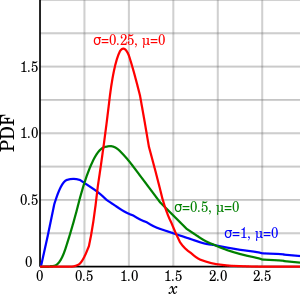
Probability density function Some log-normal density functions with identical location parameter $\mu$ but differing scale parameters $\sigma$
Cumulative distribution function Cumulative distribution function of the log-normal distribution (with $\mu = 0$ )
Notation	$\ln\mathcal{N}(\mu,\,\sigma^2)$
Parameters	$\mu \in \mathbb R$ — location, $\sigma > 0$ — scale
Support	$x \in (0, +\infty)$
PDF	$\frac{1}{x\sigma\sqrt{2\pi}}\ e^{-\frac{\left(\ln x-\mu\right)^2}{2\sigma^2}}$
CDF	$\frac12 + \frac12\,\mathrm{erf}\Big[\frac{\ln x-\mu}{\sqrt{2}\sigma}\Big]$
Mean	$e^{\mu+\sigma^2/2}$
Median	$e^{\mu}\,$
Mode	$e^{\mu-\sigma^2}$
Variance	$(e^{\sigma^2}\!\!-1) e^{2\mu+\sigma^2}$
Skewness	$(e^{\sigma^2}\!\!+2) \sqrt{e^{\sigma^2}\!\!-1}$
Ex. kurtosis	$e^{4\sigma^2}\!\! + 2e^{3\sigma^2}\!\! + 3e^{2\sigma^2}\!\! - 6$
Entropy	$\frac12 + \frac12 \ln(2\pi\sigma^2) + \mu$
MGF	(defined only on the negative half-axis, see text)
CF	representation $\sum_{n=0}^{\infty}\frac{(it)^n}{n!}e^{n\mu+n^2\sigma^2/2}$ is asymptotically divergent but sufficient for numerical purposes
Fisher information	$\begin{pmatrix}1/\sigma^2&0\\0&2/\sigma^2\end{pmatrix}$

In probability theory, a log-normal (or lognormal) distribution is a continuous probability distribution of a random variable whose logarithm is normally distributed. Thus, if the random variable $X$ is log-normally distributed, then $Y = \ln(X)$ has a normal distribution. Likewise, if $Y$ has a normal distribution, then $X = \exp(Y)$ has a log-normal distribution. A random variable which is log-normally distributed takes only positive real values.

The distribution is occasionally referred to as the Galton distribution or Galton's distribution, after Francis Galton.^[1] The log-normal distribution also has been associated with other names, such as McAlister, Gibrat and Cobb–Douglas.^[1]

A variable might be modeled as log-normal if it can be thought of as the multiplicative product of many independent random variables, each of which is positive. This is justified by considering the central limit theorem in the log domain.

For example, in finance, the variable could represent the compound return from a sequence of many trades, each expressed as its return + 1; or a long-term discount factor can be derived from the product of short-term discount factors. This was observed by Gilbrat, who claimed that the size of a firm and its growth rate are independent, and called the associated central limit tendency "the law of proportionate effect."^[2]

In wireless communication, the delay caused by shadowing or slow fading from random objects is often assumed to be log-normally distributed: see log-distance path loss model.

The log-normal distribution is the maximum entropy probability distribution for a random variate $X$ for which the mean and variance of $\ln(X)$ are specified.^[3]

Notation

Given a log-normally distributed random variable $X$ and two parameters $\mu$ and $\sigma$ that are, respectively, the mean and standard deviation of the variable’s natural logarithm (by definition, the variable’s logarithm is normally distributed), we can write $X$ as

X=e^{\mu+\sigma Z}

with $Z$ a standard normal variable.

This relationship is true regardless of the base of the logarithmic or exponential function. If $\log_a(Y)$ is normally distributed, then so is $\log_b(Y)$ , for any two positive numbers $a,b\neq 1$ . Likewise, if $e^X$ is log-normally distributed, then so is $a^{X}$ , where $a$ is a positive number $\neq 1$ .

On a logarithmic scale, $\mu$ and $\sigma$ can be called the location parameter and the scale parameter, respectively.

In contrast, the mean, standard deviation, and variance of the non-logarithmized sample values are respectively denoted $m$ , s.d., and $v$ in this article. The two sets of parameters can be related as (see also Arithmetic moments below)^[4]

\mu=\ln\left(\frac{m}{\sqrt{1+\frac{v}{m^2}}}\right), \sigma=\sqrt{\ln\left(1+\frac{v}{m^2}\right)}

Characterization

Probability density function

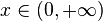
The probability density function of a log-normal distribution is:^[1]

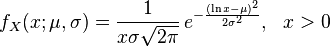
f_X(x;\mu,\sigma) = \frac{1}{ x\sigma \sqrt{2 \pi}}\, e^{-\frac{(\ln x - \mu)^2}{2\sigma^2}},\ \ x>0

This follows by applying the change-of-variables rule on the density function of a normal distribution.

Cumulative distribution function

The cumulative distribution function is

F_X(x;\mu,\sigma) = \int_{0}^{x} f_X(\xi;\mu,\sigma) d\xi = \frac12 \left[ 1 + \operatorname{erf}\!\left(\frac{\ln x - \mu}{\sigma\sqrt{2}}\right) \right] = \frac12 \operatorname{erfc}\!\left(-\frac{\ln x - \mu}{\sigma\sqrt{2}}\right) = \Phi\bigg(\frac{\ln x - \mu}{\sigma}\bigg),

where erfc is the complementary error function, and Φ is the cumulative distribution function of the standard normal distribution.

Characteristic function and moment generating function

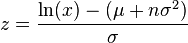All moments of the log-normal distribution exist and it holds that: $\operatorname{E}[X^n]=\mathrm{e}^{n\mu+\frac{n^2\sigma^2}{2}}$ (which can be derived by letting $z=\frac{\ln(x) - (\mu+n\sigma^2)}{\sigma}$ within the integral). However, the expected value $\operatorname{E}[e^{t X}]$ is not defined for any positive value of the argument $t$ as the defining integral diverges. In consequence the moment generating function is not defined.^[5] The last is related to the fact that the lognormal distribution is not uniquely determined by its moments.

Similarly, the characteristic function $\operatorname{E}[e^{i t X}]$ is not defined in the half complex plane and therefore it is not analytic in the origin. In consequence, the characteristic function of the log-normal distribution cannot be represented as an infinite convergent series.^[6] In particular, its Taylor formal series $\sum_{n=0}^\infty \frac{(it)^n}{n!}e^{n\mu+n^2\sigma^2/2}$ diverges. However, a number of alternative divergent series representations have been obtained^[6]^[7]^[8]^[9]

A closed-form formula for the characteristic function $\varphi(t)$ with $t$ in the domain of convergence is not known. A relatively simple approximating formula is available in closed form and given by^[10]

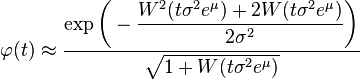
$\varphi(t)\approx\frac{\exp\bigg(-\dfrac{W^2(t\sigma^2e^\mu)+2W(t\sigma^2e^\mu)}{2\sigma^2}\bigg)}{\sqrt{1+W(t\sigma^2e^\mu)}}$

where $W$ is the Lambert W function. This approximation is derived via an asymptotic method but it stays sharp all over the domain of convergence of $\varphi$ .

Properties

Location and scale

The location and scale parameters of a log-normal distribution, i.e. $\mu$ and $\sigma$ , are more readily treated using the geometric mean, $\mathrm{GM}[X]$ , and the geometric standard deviation, $\mathrm{GSD}[X]$ , rather than the arithmetic mean, $\mathrm{E}[X]$ , and the arithmetic standard deviation, $\mathrm{SD}[X]$ .

Geometric moments

The geometric mean of the log-normal distribution is $\mathrm{GM}[X] = e^{\mu}$ , and the geometric standard deviation is $\mathrm{GSD}[X] = e^{\sigma}$ .^[11]^[12] By analogy with the arithmetic statistics, one can define a geometric variance, $\mathrm{GVar}[X] = e^{\sigma^2}$ , and a geometric coefficient of variation,^[11] $\mathrm{GCV}[X] = e^{\sigma} - 1$ .

Because the log-transformed variable $Y = \ln X$ is symmetric and quantiles are preserved under monotonic transformations, the geometric mean of a log-normal distribution is equal to its median, $\mathrm{Med}[X]$ .^[13]

Note that the geometric mean is less than the arithmetic mean. This is due to the AM–GM inequality, and corresponds to the logarithm being convex down. In fact,

\begin{align} \mathrm{E}[X] &= e^{\mu + \frac12 \sigma^2} &= e^{\mu} \cdot \sqrt{e^{\sigma^2}} &= \mathrm{GM}[X] \cdot \sqrt{\mathrm{GVar}[X]}. \end{align}

In finance the term $e^{-\frac12\sigma^2}$ is sometimes interpreted as a convexity correction. From the point of view of stochastic calculus, this is the same correction term as in Itō's lemma for geometric Brownian motion.

Arithmetic moments

The arithmetic mean, arithmetic variance, and arithmetic standard deviation of a log-normally distributed variable $X$ are given by

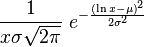
\begin{align} & \operatorname{E}[X] = e^{\mu + \tfrac{1}{2}\sigma^2}, \\ & \operatorname{Var}[X] = (e^{\sigma^2} - 1) e^{2\mu + \sigma^2} = (e^{\sigma^2} - 1)(\operatorname{E}[X])^2, \\ & \operatorname{SD}[X] = \sqrt{\operatorname{Var}[X]} = e^{\mu + \tfrac{1}{2}\sigma^2}\sqrt{e^{\sigma^2} - 1} = \operatorname{E}[X] \sqrt{e^{\sigma^2} - 1}, \end{align}

respectively.

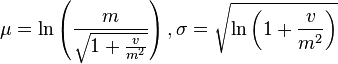
The location ( $\mu$ ) and scale ( $\sigma$ ) parameters can be obtained if the arithmetic mean and the arithmetic variance are known; it is simpler if $\sigma$ is computed first:

\begin{align} \mu &= \ln(\operatorname{E}[X]) - \frac12 \ln\!\left(1 + \frac{\mathrm{Var}[X]}{(\operatorname{E}[X])^2}\right) = \ln(\operatorname{E}[X]) - \frac12 \sigma^2, \\ \sigma^2 &= \ln\!\left(1 + \frac{\operatorname{Var}[X]}{(\operatorname{E}[X])^2}\right). \end{align}

For any real or complex number $s$ , the $s$ ^th moment of a log-normally distributed variable $X$ is given by^[1]

\operatorname{E}[X^s] = e^{s\mu + \frac12s^2\sigma^2}.

A log-normal distribution is not uniquely determined by its moments $\operatorname{E}[X^k]$ for $k\geq1$ , that is, there exists some other distribution with the same moments for all $k$ .^[1] In fact, there is a whole family of distributions with the same moments as the log-normal distribution.

Mode and median

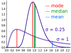
Comparison of mean, median and mode of two log-normal distributions with different skewness.

The mode is the point of global maximum of the probability density function. In particular, it solves the equation $(\ln f)'=0$ :

\mathrm{Mode}[X] = e^{\mu - \sigma^2}.

The median is such a point where $F_X=0.5$ :

\mathrm{Med}[X] = e^\mu\,.

Arithmetic coefficient of variation

The arithmetic coefficient of variation $\mathrm{CV}[X]$ is the ratio $\frac{\mathrm{SD}[X]}{\mathrm{E}[X]}$ (on the natural scale). For a log-normal distribution it is equal to

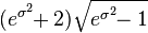
\mathrm{CV}[X] = \sqrt{e^{\sigma^2} - 1}.

Contrary to the arithmetic standard deviation, the arithmetic coefficient of variation is independent of the arithmetic mean.

Partial expectation

The partial expectation of a random variable $X$ with respect to a threshold $k$ is defined as 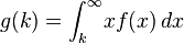$g(k) = \int_k^\infty \!xf(x)\, dx$ where $f(x)$ is the probability density function of $X$ . Alternatively, and using the definition of conditional expectation, it can be written as $g(k)=\operatorname{E}[X|X>k] P(X>k)$ . For a log-normal random variable the partial expectation is given by:

g(k) = \int_k^\infty \!xf(x)\, dx = e^{\mu+\tfrac{1}{2}\sigma^2}\, \Phi\!\left(\frac{\mu+\sigma^2-\ln k}{\sigma}\right).

Where Phi is the normal cumulative distribution function. The derivation of the formula is provided in the discussion of this Wikipedia entry. The partial expectation formula has applications in insurance and economics, it is used in solving the partial differential equation leading to the Black–Scholes formula.

Other

A set of data that arises from the log-normal distribution has a symmetric Lorenz curve (see also Lorenz asymmetry coefficient).^[14]

The harmonic $H$ , geometric $G$ and arithmetic $A$ means of this distribution are related;^[15] such relation is given by

H = \frac{G^2}{ A} .

Log-normal distributions are infinitely divisible.^[1]

Occurrence

The log-normal distribution is important in the description of natural phenomena. The reason is that for many natural processes of growth, growth rate is independent of size. This is also known as Gibrat's law, after Robert Gibrat (1904–1980) who formulated it for companies. It can be shown that a growth process following Gibrat's law will result in entity sizes with a log-normal distribution.^[16] Examples include:

In biology and medicine,
- Measures of size of living tissue (length, skin area, weight);^[17]
- For highly communicable epidemics, such as SARS in 2003, if publication intervention is involved, the number of hospitalized cases is shown to satistfy the lognormal distribution with no free parameters if an entropy is assumed and the standard deviation is determined by the principle of maximum rate of entropy production.^[18]
- The length of inert appendages (hair, claws, nails, teeth) of biological specimens, in the direction of growth;
- Certain physiological measurements, such as blood pressure of adult humans (after separation on male/female subpopulations)^[19]

Fitted cumulative log-normal distribution to annually maximum 1-day rainfalls, see distribution fitting

Consequently, reference ranges for measurements in healthy individuals are more accurately estimated by assuming a log-normal distribution than by assuming a symmetric distribution about the mean.

In colloidal chemistry and polymer chemistry
- Particle size distributions
- Molar mass distributions

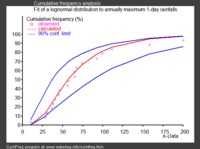
In hydrology, the log-normal distribution is used to analyze extreme values of such variables as monthly and annual maximum values of daily rainfall and river discharge volumes.^[20]
- The image on the right illustrates an example of fitting the log-normal distribution to ranked annually maximum one-day rainfalls showing also the 90% confidence belt based on the binomial distribution. The rainfall data are represented by plotting positions as part of a cumulative frequency analysis.

In social sciences and demographics
- In economics, there is evidence that the income of 97%–99% of the population is distributed log-normally.^[21] (The distribution of higher-income individuals follows a Pareto distribution.^[22])
- In finance, in particular the Black–Scholes model, changes in the logarithm of exchange rates, price indices, and stock market indices are assumed normal^[23] (these variables behave like compound interest, not like simple interest, and so are multiplicative). However, some mathematicians such as Benoît Mandelbrot have argued ^[24] that log-Lévy distributions which possesses heavy tails would be a more appropriate model, in particular for the analysis for stock market crashes. Indeed stock price distributions typically exhibit a fat tail.^[25]
- city sizes

Technology
- In reliability analysis, the lognormal distribution is often used to model times to repair a maintainable system.^[26]
- In wireless communication, "the local-mean power expressed in logarithmic values, such as dB or neper, has a normal (i.e., Gaussian) distribution." ^[27] Also, the random obstruction of radio signals due to large buildings and hills, called shadowing, is often modeled as a lognormal distribution.
- It has been proposed that coefficients of friction and wear may be treated as having a lognormal distribution ^[28]
- In spray process, such as droplet impact, the size of secondary produced droplet has a lognormal distribution, with the standard deviation ： $\sigma=\frac{\sqrt{6}}{6}$ determined by the principle of maximum rate of entropy production^[29] If the lognormal distribution is inserted into the Shannon entropy expression and if the rate of entropy production is maximized (principle of maximum rate of entropy production), then σ is given by : $\sigma=\frac{1}{\sqrt{6}}$ ^[29] and with this parameter the droplet size distribution for spray process is well predicted. It is an open question whether this value of σ has some generality for other cases, though for spreading of communicable epidemics, σ is shown also to take this value.^[18]
- Particle size distributions produced by comminution with random impacts, such as in ball milling
- The file size distribution of publicly available audio and video data files (MIME types) follows a log-normal distribution over five orders of magnitude.^[30]

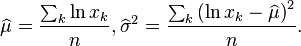
Maximum likelihood estimation of parameters

For determining the maximum likelihood estimators of the log-normal distribution parameters μ and σ, we can use the same procedure as for the normal distribution. To avoid repetition, we observe that

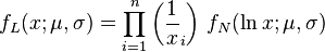
f_L (x;\mu, \sigma) = \prod_{i=1}^n \left(\frac 1 x_i\right) \, f_N (\ln x; \mu, \sigma)

where by $f_L$ we denote the probability density function of the log-normal distribution and by $f_N$ that of the normal distribution. Therefore, using the same indices to denote distributions, we can write the log-likelihood function thus:

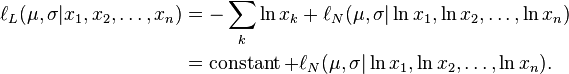
\begin{align} \ell_L (\mu,\sigma | x_1, x_2, \dots, x_n) & {} = - \sum _k \ln x_k + \ell_N (\mu, \sigma | \ln x_1, \ln x_2, \dots, \ln x_n) \\ & {} = \operatorname {constant} + \ell_N (\mu, \sigma | \ln x_1, \ln x_2, \dots, \ln x_n). \end{align}

Since the first term is constant with regard to μ and σ, both logarithmic likelihood functions, $\ell_L$ and $\ell_N$ , reach their maximum with the same $\mu$ and $\sigma$ . Hence, using the formulas for the normal distribution maximum likelihood parameter estimators and the equality above, we deduce that for the log-normal distribution it holds that

\widehat \mu = \frac {\sum_k \ln x_k} n, \widehat \sigma^2 = \frac {\sum_k \left( \ln x_k - \widehat \mu \right)^2} {n}.

Multivariate log-normal

If $\boldsymbol X \sim \mathcal{N}(\boldsymbol\mu,\,\boldsymbol\Sigma)$ is a multivariate normal distribution then $\boldsymbol Y=\exp(\boldsymbol X)$ has a multivariate log-normal distribution^[31] with mean

\operatorname{E}[\boldsymbol Y]_i=e^{\mu_i+\frac{1}{2}\Sigma_{ii}} ,

and covariance matrix

\operatorname{Var}[\boldsymbol Y]_{ij}=e^{\mu_i+\mu_j + \frac{1}{2}(\Sigma_{ii}+\Sigma_{jj}) }( e^{\Sigma_{ij}} - 1) .

Related distributions

If $X \sim \mathcal{N}(\mu, \sigma^2)$ is a normal distribution, then $\exp(X) \sim \operatorname{\ln\mathcal{N}}(\mu, \sigma^2).$

If $X \sim \operatorname{\ln\mathcal{N}}(\mu, \sigma^2)$ is distributed log-normally, then $\ln(X) \sim \mathcal{N}(\mu, \sigma^2)$ is a normal random variable.

If $X_j \sim \operatorname{\ln\mathcal{N}}(\mu_j, \sigma_j^2)$ are $n$ independent log-normally distributed variables, and $Y = \textstyle\prod_{j=1}^n X_j$ , then $Y$ is also distributed log-normally:

Y \sim \operatorname{\ln\mathcal{N}}\Big(\textstyle \sum_{j=1}^n\mu_j,\ \sum_{j=1}^n \sigma_j^2 \Big).

Let $X_j \sim \operatorname{\ln\mathcal{N}}(\mu_j,\sigma_j^2)\$ be independent log-normally distributed variables with possibly varying $\sigma$ and $\mu$ parameters, and $Y=\textstyle\sum_{j=1}^n X_j$ . The distribution of $Y$ has no closed-form expression, but can be reasonably approximated by another log-normal distribution $Z$ at the right tail.^[32] Its probability density function at the neighborhood of 0 has been characterized^[33] and it does not resemble any log-normal distribution. A commonly used approximation due to L.F. Fenton (but previously stated by R.I. Wilkinson and mathematical justified by Marlow^[34]) is obtained by matching the mean and variance of another lognormal distribution:

\begin{align} \sigma^2_Z &= \ln\!\left[ \frac{\sum e^{2\mu_j+\sigma_j^2}(e^{\sigma_j^2}-1)}{(\sum e^{\mu_j+\sigma_j^2/2})^2} + 1\right], \\ \mu_Z &= \ln\!\left[ \sum e^{\mu_j+\sigma_j^2/2} \right] - \frac{\sigma^2_Z}{2}. \end{align}

In the case that all $X_j$ have the same variance parameter $\sigma_j=\sigma$ , these formulas simplify to

\begin{align} \sigma^2_Z &= \ln\!\left[ (e^{\sigma^2}-1)\frac{\sum e^{2\mu_j}}{(\sum e^{\mu_j})^2} + 1\right], \\ \mu_Z &= \ln\!\left[ \sum e^{\mu_j} \right] + \frac{\sigma^2}{2} - \frac{\sigma^2_Z}{2}. \end{align}

If $X \sim \operatorname{\ln\mathcal{N}}(\mu, \sigma^2)$ , then $X+c$ is said to have a shifted log-normal distribution with support $x\in (c, +\infty)$ . $\operatorname{E}[X+c] = \operatorname{E}[X]+c$ , $\operatorname{Var}[X+c] = \operatorname{Var}[X]$ .

If $X \sim \operatorname{\ln\mathcal{N}}(\mu, \sigma^2)$ , then $a X \sim \operatorname{\ln\mathcal{N}}( \mu + \ln a,\ \sigma^2).$

If $X \sim \operatorname{\ln\mathcal{N}}(\mu, \sigma^2)$ , then $\tfrac{1}{X} \sim \operatorname{\ln\mathcal{N}}(-\mu,\ \sigma^2).$

If $X \sim \operatorname{\ln\mathcal{N}}(\mu, \sigma^2)$ then $X^a \sim \operatorname{\ln\mathcal{N}}(a\mu,\ a^2 \sigma^2).$ for $a \neq 0\,$

Lognormal distribution is a special case of semi-bounded Johnson distribution

If $X|Y \sim \mathrm{Rayleigh}(Y)\,$ with $Y \sim \operatorname{\ln\mathcal{N}}(\mu, \sigma^2)$ , then $X \sim \mathrm{Suzuki}(\mu, \sigma)\,$ (Suzuki distribution)

Similar distributions

A substitute for the log-normal whose integral can be expressed in terms of more elementary functions^[35] can be obtained based on the logistic distribution to get an approximation for the CDF

F(x;\mu,\sigma) = \left[\left(\frac{e^\mu}{x}\right)^{\pi/(\sigma \sqrt{3})} +1\right]^{-1}.

This is a log-logistic distribution.

Notes

↑ 1.0 1.1 1.2 1.3 1.4 1.5 Johnson, Norman L.; Kotz, Samuel; Balakrishnan, N. (1994), "14: Lognormal Distributions", Continuous univariate distributions. Vol. 1, Wiley Series in Probability and Mathematical Statistics: Applied Probability and Statistics (2nd ed.), New York: John Wiley & Sons, ISBN 978-0-471-58495-7, MR 1299979
↑ Kunio Shimizu and Edwin L. Crow, "History, Genesis, and Properties", ch. 1 in Crow and Shimizu (1988)
↑ Park, Sung Y.; Bera, Anil K. (2009). "Maximum entropy autoregressive conditional heteroskedasticity model" (PDF). Journal of Econometrics (Elsevier) 150 (2): 219–230. doi:10.1016/j.jeconom.2008.12.014. Retrieved 2011-06-02.
↑ "Lognormal mean and variance"
↑ Heyde, CC. (1963), "On a property of the lognormal distribution", Journal of the Royal Statistical Society, Series B (Methodological) 25 (2): 392–393, doi:10.1007/978-1-4419-5823-5_6
↑ 6.0 6.1 Holgate, P. (1989). "The lognormal characteristic function, vol. 18, pp. 4539–4548, 1989". Communications in Statistical – Theory and Methods 18 (12): 4539–4548. doi:10.1080/03610928908830173.
↑ Barakat, R. (1976). "Sums of independent lognormally distributed random variables". Journal of the Optical Society of America 66 (3): 211–216. doi:10.1364/JOSA.66.000211.
↑ Barouch, E.; Kaufman, GM.; Glasser, ML. (1986). "On sums of lognormal random variables" (PDF). Studies in Applied Mathematics 75 (1): 37–55.
↑ Leipnik, Roy B. (January 1991). "On Lognormal Random Variables: I – The Characteristic Function". Journal of the Australian Mathematical Society Series B 32 (3): 327–347. doi:10.1017/S0334270000006901.
↑ S. Asmussen, J.L. Jensen, L. Rojas-Nandayapa. "On the Laplace transform of the Lognormal distribution", Thiele centre preprint, (2013).
↑ 11.0 11.1 Kirkwood, Thomas BL (Dec 1979). "Geometric means and measures of dispersion". Biometrics 35 (4): 908–9. doi:10.2307/2530139.
↑ Limpert, E; Stahel, W; Abbt, M (2001). "Lognormal distributions across the sciences: keys and clues". BioScience 51 (5): 341–352. doi:10.1641/0006-3568(2001)051[0341:LNDATS]2.0.CO;2.
↑ Daly, Leslie E.; Bourke, Geoffrey Joseph (2000). Interpretation and uses of medical statistics (5th ed.). Wiley-Blackwell. p. 89. doi:10.1002/9780470696750. ISBN 978-0-632-04763-5.
↑ Damgaard, Christian; Weiner, Jacob (2000). "Describing inequality in plant size or fecundity". Ecology 81 (4): 1139–1142. doi:10.1890/0012-9658(2000)081[1139:DIIPSO]2.0.CO;2.
↑ Rossman, Lewis A (July 1990). "Design stream ﬂows based on harmonic means". J Hydraulic Engineering 116 (7): 946–950. doi:10.1061/(ASCE)0733-9429(1990)116:7(946).
↑ Sutton, John (Mar 1997). "Gibrat's Legacy". Journal of Economic Literature 32 (1): 40–59. JSTOR 2729692.
↑ Huxley, Julian S. (1932). Problems of relative growth. London. ISBN 0-486-61114-0. OCLC 476909537.
↑ 18.0 18.1 Wang, WB; Wang, CF; Wu, ZN; Hu, RF (2013). "Modelling the spreading rate of controlled communicable epidemics through an entropy-based thermodynamic model" 56 (11). SCIENCE CHINA Physics, Mechanics & Astronomy. pp. 2143–2150.
↑ Makuch, Robert W.; D.H. Freeman, M.F. Johnson (1979). "Justification for the lognormal distribution as a model for blood pressure". Journal of Chronic Diseases 32 (3): 245–250. doi:10.1016/0021-9681(79)90070-5. Retrieved 27 February 2012.
↑ Ritzema (ed.), H.P. (1994). Frequency and Regression Analysis (PDF). Chapter 6 in: Drainage Principles and Applications, Publication 16, International Institute for Land Reclamation and Improvement (ILRI), Wageningen, The Netherlands. pp. 175–224. ISBN 90-70754-33-9.
↑ Clementi, Fabio; Gallegati, Mauro (2005) "Pareto's law of income distribution: Evidence for Germany, the United Kingdom, and the United States", EconWPA
↑ Wataru, Souma (2002-02-22). "Physics of Personal Income". arXiv:cond-mat/0202388.
↑ Black, F.; Scholes, M. (1973). "The Pricing of Options and Corporate Liabilities". Journal of Political Economy 81 (3): 637. doi:10.1086/260062.
↑ Mandelbrot, Benoit (2004). The (mis-)Behaviour of Markets. Basic Books. ISBN 9780465043552.
↑ Bunchen, P., Advanced Option Pricing, University of Sydney coursebook, 2007
↑ O'Connor, Patrick; Kleyner, Andre (2011). Practical Reliability Engineering. John Wiley & Sons. p. 35. ISBN 978-0-470-97982-2.
↑ http://wireless.per.nl/reference/chaptr03/shadow/shadow.htm
↑ Steele, C. (2008). "Use of the lognormal distribution for the coefficients of friction and wear". Reliability Engineering & System Safety 93 (10): 1574–2013. doi:10.1016/j.ress.2007.09.005.
↑ 29.0 29.1 Wu, Zi-Niu (July 2003). "Prediction of the size distribution of secondary ejected droplets by crown splashing of droplets impinging on a solid wall". Probabilistic Engineering Mechanics 18 (3): 241–249. doi:10.1016/S0266-8920(03)00028-6.
↑ Gros, C; Kaczor, G.; Markovic, D (2012). "Neuropsychological constraints to human data production on a global scale". The European Physical Journal B 85 (28). doi:10.1140/epjb/e2011-20581-3.
↑ Tarmast, Ghasem (2001). Multivariate Log–Normal Distribution (PDF). ISI Proceedings: 53rd Session. Seoul.
↑ Asmussen, S.; Rojas-Nandayapa, L. (2008). "Asymptotics of Sums of Lognormal Random Variables with Gaussian Copula". Statistics and Probability Letters 78 (16): 2709–2714. doi:10.1016/j.spl.2008.03.035.
↑ Gao, X.; Xu, H; Ye, D. (2009), "Asymptotic Behaviors of Tail Density for Sum of Correlated Lognormal Variables". International Journal of Mathematics and Mathematical Sciences, vol. 2009, Article ID 630857. doi:10.1155/2009/630857
↑ Marlow, NA. (Nov 1967). "A normal limit theorem for power sums of independent normal random variables". Bell System Technical Journal 46 (9): 2081–2089. doi:10.1002/j.1538-7305.1967.tb04244.x.
↑ Swamee, P. K. (2002). "Near Lognormal Distribution". Journal of Hydrologic Engineering 7 (6): 441–444. doi:10.1061/(ASCE)1084-0699(2002)7:6(441).

References

Crow, Edwin L.; Shimizu, Kunio (Editors) (1988), Lognormal Distributions, Theory and Applications, Statistics: Textbooks and Monographs 88, New York: Marcel Dekker, Inc., pp. xvi+387, ISBN 0-8247-7803-0, MR 0939191, Zbl 0644.62014
Aitchison, J. and Brown, J.A.C. (1957) The Lognormal Distribution, Cambridge University Press.
E. Limpert, W. Stahel and M. Abbt (2001) Log-normal Distributions across the Sciences: Keys and Clues, BioScience, 51 (5), 341–352.
Eric W. Weisstein et al. Log Normal Distribution at MathWorld. Electronic document, retrieved October 26, 2006.

Holgate, P. (1989). "The lognormal characteristic function". Communications in Statistics - Theory and Methods 18 (12): 4539–4548. doi:10.1080/03610928908830173.

External links

Wikimedia Commons has media related to Log-normal distribution.

Probability distributions

Discrete univariate with finite support

Benford Bernoulli Beta-binomial binomial categorical hypergeometric Poisson binomial Rademacher discrete uniform Zipf Zipf–Mandelbrot

Discrete univariate with infinite support

beta negative binomial Borel Conway–Maxwell–Poisson discrete phase-type Delaporte extended negative binomial Gauss–Kuzmin geometric logarithmic negative binomial parabolic fractal Poisson Skellam Yule–Simon zeta

Continuous univariate supported on a bounded interval, e.g. [0,1]

Arcsine ARGUS Balding–Nichols Bates Beta Beta rectangular Irwin–Hall Kumaraswamy logit-normal Noncentral beta raised cosine Triangular U-quadratic uniform Wigner semicircle

[[List of probability distributions#Supported_on_semi-infinite_intervals.2C_usually_.5B0.2C.E2.88.9E.29|Continuous univariate supported on a semi-infinite interval, usually [0,∞)]]

Benini
Benktander 1st kind
Benktander 2nd kind
Beta prime
Burr
chi-squared
chi
Coxian
Dagum
Davis
EL
Erlang
exponential
F
folded normal
Flory-Schulz
Fréchet
Gamma
Gamma/Gompertz
generalized inverse Gaussian
Gompertz
half-logistic
half-normal
Hotelling's T-squared
hyper-Erlang
hyperexponential
hypoexponential
inverse chi-squared (scaled inverse chi-squared)
inverse Gaussian
inverse gamma
Kolmogorov
Lévy
log-Cauchy
log-Laplace
log-logistic
log-normal
matrix-exponential
Maxwell–Boltzmann
Maxwell–Jüttner
Mittag–Leffler
Nakagami
noncentral chi-squared
Pareto
phase-type
Poly-Weibull
Rayleigh
relativistic Breit–Wigner
Rice
Rosin–Rammler
shifted Gompertz
truncated normal
type-2 Gumbel
Weibull
Wilks' lambda

Continuous univariate supported on the whole real line (−∞, ∞)

Cauchy exponential power Fisher's z generalized normal generalized hyperbolic geometric stable Gumbel Holtsmark hyperbolic secant Johnson SU Landau Laplace Linnik logistic noncentral t normal (Gaussian) normal-inverse Gaussian skew normal slash stable Student's t type-1 Gumbel Tracy–Widom variance-gamma Voigt

Continuous univariate with support whose type varies

generalized extreme value generalized Pareto Tukey lambda q-Gaussian q-exponential q-Weibull shifted log-logistic

Mixed continuous-discrete univariate distributions

rectified Gaussian

Multivariate (joint)

Discrete Ewens multinomial Dirichlet-multinomial negative multinomial Continuous Dirichlet Generalized Dirichlet multivariate normal Multivariate stable multivariate Student normal-scaled inverse gamma normal-gamma Matrix-valued inverse matrix gamma inverse-Wishart matrix normal matrix t matrix gamma normal-inverse-Wishart normal-Wishart Wishart

Directional

Univariate (circular) directional Circular uniform univariate von Mises wrapped normal wrapped Cauchy wrapped exponential wrapped Lévy Bivariate (spherical) Kent Bivariate (toroidal) bivariate von Mises Multivariate von Mises–Fisher Bingham

Degenerate and singular

Degenerate discrete degenerate Dirac delta function Singular Cantor

Families

Circular compound Poisson elliptical exponential natural exponential location-scale maximum entropy mixture Pearson Tweedie wrapped

Some common univariate probability distributions

Continuous	beta Cauchy chi-squared exponential F gamma Laplace log-normal normal Pareto Student's t uniform Weibull

Discrete	Bernoulli binomial discrete uniform geometric hypergeometric negative binomial Poisson

List of probability distributions