Location estimation in sensor networks
Location estimation in wireless sensor networks is the problem of estimating the location of an object from a set of noisy measurements. These measurements are acquired in a distributed manner by a set of sensors.
Motivation
Many civilian and military applications require monitoring that can identify objects in a specific area, such as monitoring the front entrance of a private house by a single camera. Monitored areas that are large relative to objects of interest often require multiple sensors (e.g., infra-red detectors) at multiple locations. A centralized observer or computer application monitors the sensors. The communication to power and bandwidth requirements call for efficient design of the sensor, transmission, and processing.
The CodeBlue system of Harvard university is an example where a vast number of sensors distributed among hospital facilities allow staff to locate a patient in distress. In addition, the sensor array enables online recording of medical information while allowing the patient to move around. Military applications (e.g. locating an intruder into a secured area) are also good candidates for setting a wireless sensor network.
Setting
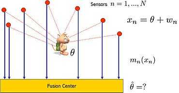
Let  denote the position of interest. A set of
  sensors
acquire measurements
sensors
acquire measurements  contaminated by an
additive noise
contaminated by an
additive noise  owing some known or unknown probability density function (PDF). The sensors transmit measurements to a central processor. The
  th sensor encodes
 by a function
  . The application processing the data applies a pre-defined estimation rule
 . The set of message functions
 and the fusion rule
 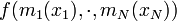 are
designed to minimize estimation error.
For example: minimizing the mean squared error (MSE),
are
designed to minimize estimation error.
For example: minimizing the mean squared error (MSE),
 .
.
Ideally, sensors transmit their measurements
right to the processing center, that is 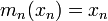 . In this
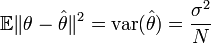
settings, the maximum likelihood estimator (MLE)
. In this
settings, the maximum likelihood estimator (MLE) 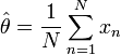 is an unbiased estimator whose MSE is
 assuming a white Gaussian noise
 . The next sections suggest
alternative designs when the sensors are bandwidth constrained to
1 bit transmission, that is =0 or 1.
. The next sections suggest
alternative designs when the sensors are bandwidth constrained to
1 bit transmission, that is =0 or 1.
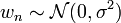
Known noise PDF
We begin with an example of a Gaussian noise
, in which a suggestion for a
system design is as follows
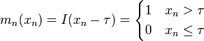
Here  is a parameter leveraging our prior knowledge of the
approximate location of . In this design, the random value
of is distributed Bernoulli~
is a parameter leveraging our prior knowledge of the
approximate location of . In this design, the random value
of is distributed Bernoulli~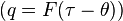 . The
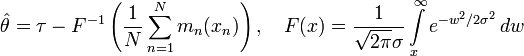
processing center averages the received bits to form an estimate
. The
processing center averages the received bits to form an estimate
 of
of  , which is then used to find an estimate of . It can be verified that for the optimal (and
infeasible) choice of
, which is then used to find an estimate of . It can be verified that for the optimal (and
infeasible) choice of  the variance of this estimator
is
the variance of this estimator
is  which is only
  times the
variance of MLE without bandwidth constraint. The variance
increases as deviates from the real value of , but it can be shown that as long as
times the
variance of MLE without bandwidth constraint. The variance
increases as deviates from the real value of , but it can be shown that as long as  the factor in the MSE remains approximately 2. Choosing a suitable value for is a major disadvantage of this method since our model does not assume prior knowledge about the approximated location of . A coarse estimation can be used to overcome this limitation. However, it requires additional hardware in each of
the sensors.
the factor in the MSE remains approximately 2. Choosing a suitable value for is a major disadvantage of this method since our model does not assume prior knowledge about the approximated location of . A coarse estimation can be used to overcome this limitation. However, it requires additional hardware in each of
the sensors.
A system design with arbitrary (but known) noise PDF can be found in.[2] In this setting it is assumed that both and
the noise are confined to some known interval ![[-U,U]](../I/m/3d08f01949bb41891d359638fa72ad13.png) . The
estimator of [2] also reaches an MSE which is a constant factor
times
. The
estimator of [2] also reaches an MSE which is a constant factor
times  . In this method, the prior knowledge of
  replaces
the parameter of the previous approach.
replaces
the parameter of the previous approach.
Unknown noise parameters
A noise model may be sometimes available while the exact PDF parameters are unknown (e.g. a Gaussian PDF with unknown  ). The idea proposed in [3] for this setting is to use two
thresholds
). The idea proposed in [3] for this setting is to use two
thresholds  , such that
  sensors are designed
with
sensors are designed
with 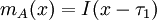 , and the other sensors use
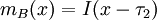 . The processing center estimation rule is generated as follows:
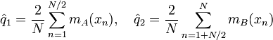
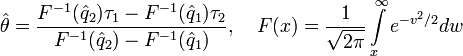
As before, prior knowledge is necessary to set values for
to have an MSE with a reasonable factor
of the unconstrained MLE variance.
Unknown noise PDF
We now describe the system design of [2] for the case that the structure of the noise PDF is unknown. The following model is considered for this scenario:

![w_n\in\mathcal{P}, \text{ that is }: w_n \text{ is bounded to }
[-U,U], \mathbb{E}(w_n)=0](../I/m/56f846c52bf74e3888833ab1ffcb4b12.png)
In addition, the message functions are limited to have the form
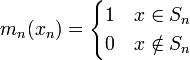
where each  is a subset of
 ![[-2U,2U]](../I/m/204c9aaba2398fcf04c876537c08cb07.png) . The fusion estimator is also restricted to be linear, i.e.
. The fusion estimator is also restricted to be linear, i.e.
 .
.
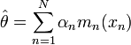
The design should set the decision intervals and the
coefficients  . Intuitively, we would allocate sensors to encode the first bit of by setting their decision interval to be
 ![[0,2U]](../I/m/45aa2c80e8c5867d7b1865aa03b584c7.png) , then
, then  sensors would encode the second bit by setting their decision interval to
![[-U,0]\cup[U,2U]](../I/m/9af54dda9318695852cde975a841b000.png) and so on. It can be shown that these decision
intervals and the corresponding set of coefficients
produce a universal
and so on. It can be shown that these decision
intervals and the corresponding set of coefficients
produce a universal  -unbiased estimator, which is an
estimator satisfying
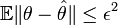
-unbiased estimator, which is an
estimator satisfying 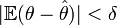 for every possible value of
 ![\theta\in[-U,U]](../I/m/c4aba35b775aa922f82c0f9c7d54f268.png) and for every realization of
and for every realization of  . In fact, this intuitive
design of the decision intervals is also optimal in the following
sense. The above design requires
. In fact, this intuitive
design of the decision intervals is also optimal in the following
sense. The above design requires
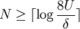 to satisfy the universal
-unbiased property while theoretical arguments show that
an optimal (and a more complex) design of the decision intervals
would require
to satisfy the universal
-unbiased property while theoretical arguments show that
an optimal (and a more complex) design of the decision intervals
would require 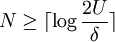 , that is:
the number of sensors is nearly optimal. It is also argued in [2]
that if the targeted MSE
, that is:
the number of sensors is nearly optimal. It is also argued in [2]
that if the targeted MSE
 uses a small
enough
uses a small
enough  , then this design requires a factor of 4 in the
number of sensors to achieve the same variance of the MLE in
the unconstrained bandwidth settings.
, then this design requires a factor of 4 in the
number of sensors to achieve the same variance of the MLE in
the unconstrained bandwidth settings.
Additional information
The design of the sensor array requires optimizing the power
allocation as well as minimizing the communication traffic of the
entire system. The design suggested in [4] incorporates probabilistic quantization in
sensors and a simple optimization program that is solved in the
fusion center only once. The fusion center then broadcasts a set
of parameters to the sensors that allows them to finalize their
design of messaging functions  as to meet the energy
constraints. Another work employs a similar approach to address
distributed detection in wireless sensor arrays.[5]
as to meet the energy
constraints. Another work employs a similar approach to address
distributed detection in wireless sensor arrays.[5]
External links
- CodeBlue Harvard group working on wireless sensor network technology to a range of medical applications.
References
- ↑ Ribeiro, Alejandro; Georgios B. Giannakis (March 2006). "Bandwidth-constrained distributed estimation for wireless sensor Networks-part I: Gaussian case". IEEE Trans. On Sig. Proc.
- ↑ 2.0 2.1 2.2 2.3 Luo, Zhi-Quan (June 2005). "Universal decentralized estimation in a bandwidth constrained sensor network". IEEE Trans. On Inf. Th.
- ↑ Ribeiro, Alejandro; Georgios B. Giannakis (July 2006). "Bandwidth-constrained distributed estimation for wireless sensor networks-part II: unknown probability density function". IEEE Trans. On Sig. Proc.
- ↑ Xiao, Jin-Jun; Andrea J. Goldsmith (June 2005). "Joint estimation in sensor networks under energy constraint". IEEE Trans. On Sig. Proc.
- ↑ Xiao, Jin-Jun; Zhi-Quan Luo (August 2005). "Universal decentralized detection in a bandwidth-constrained sensor network". IEEE Trans. On Sig. Proc.
| ||||||||||||||||||||||||||||||||||