Lissajous curve
In mathematics, a Lissajous curve /ˈlɪsəʒuː/, also known as Lissajous figure or Bowditch curve /ˈbaʊdɪtʃ/, is the graph of a system of parametric equations

which describe complex harmonic motion. This family of curves was investigated by Nathaniel Bowditch in 1815, and later in more detail by Jules Antoine Lissajous in 1857.
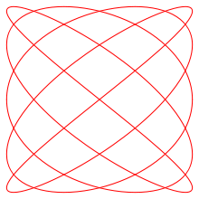
The appearance of the figure is highly sensitive to the ratio a/b. For a ratio of 1, the figure is an ellipse, with special cases including circles (A = B, δ = π/2 radians) and lines (δ = 0). Another simple Lissajous figure is the parabola (a/b = 2, δ = π/4). Other ratios produce more complicated curves, which are closed only if a/b is rational. The visual form of these curves is often suggestive of a three-dimensional knot, and indeed many kinds of knots, including those known as Lissajous knots, project to the plane as Lissajous figures.
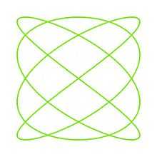
Visually, the ratio a/b determines the number of "lobes" of the figure. For example, a ratio of 3/1 or 1/3 produces a figure with three major lobes (see image). Similarly, a ratio of 5/4 produces a figure with five horizontal lobes and four vertical lobes. Rational ratios produce closed (connected) or "still" figures, while irrational ratios produce figures that appear to rotate. The ratio A/B determines the relative width-to-height ratio of the curve. For example, a ratio of 2/1 produces a figure that is twice as wide as it is high. Finally, the value of δ determines the apparent "rotation" angle of the figure, viewed as if it were actually a three-dimensional curve. For example, δ=0 produces x and y components that are exactly in phase, so the resulting figure appears as an apparent three-dimensional figure viewed from straight on (0°). In contrast, any non-zero δ produces a figure that appears to be rotated, either as a left/right or an up/down rotation (depending on the ratio a/b).
.jpg)
Lissajous figures where a = 1, b = N (N is a natural number) and
are Chebyshev polynomials of the first kind of degree N. This property is exploited to produce a set of points, called Padua points, at which a function may be sampled in order to compute either a bivariate interpolation or quadrature of the function over the domain [-1,1]×[-1,1].
Examples
The animation below shows the curve adaptation with continuously increasing  fraction from 0 to 1 in steps of 0.01. (δ=0)
Below are examples of Lissajous figures with δ = π/2, an odd natural number a, an even natural number b, and |a − b| = 1.
-
 a = 1, b = 2 (1:2)
 -
 a = 3, b = 2 (3:2)
 -
 a = 3, b = 4 (3:4)
 -
 a = 5, b = 4 (5:4)
Generation
Prior to modern electronic equipment, Lissajous curves could be generated mechanically by means of a harmonograph.
Practical application
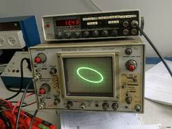
Lissajous curves can also be generated using an oscilloscope (as illustrated). An octopus circuit can be used to demonstrate the waveform images on an oscilloscope. Two phase-shifted sinusoid inputs are applied to the oscilloscope in X-Y mode and the phase relationship between the signals is presented as a Lissajous figure.
In the professional audio world, this method is used for realtime analysis of the phase relationship between the left and right channels of a stereo audio signal. On larger, more sophisticated audio mixing consoles an oscilloscope may be built-in for this purpose.
On an oscilloscope, we suppose x is CH1 and y is CH2, A is amplitude of CH1 and B is amplitude of CH2, a is frequency of CH1 and b is frequency of CH2, so a/b is a ratio of frequency of two channels, finally, δ is the phase shift of CH1.
A purely mechanical application of a Lissajous curve with a=1, b=2 is in the driving mechanism of the Mars Light type of oscillating beam lamps popular with railroads in the mid-1900s. The beam in some versions traces out a lopsided figure-8 pattern with the "8" lying on its side.
Application for the case of a = b
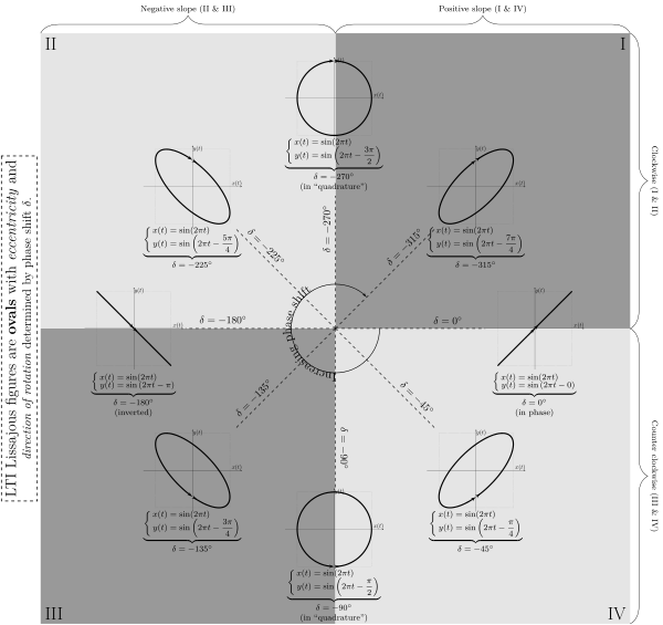
When the input to an LTI system is sinusoidal, the output is sinusoidal with the same frequency, but it may have a different amplitude and some phase shift. Using an oscilloscope that can plot one signal against another (as opposed to one signal against time) to plot the output of an LTI system against the input to the LTI system produces an ellipse that is a Lissajous figure for the special case of a = b. The aspect ratio of the resulting ellipse is a function of the phase shift between the input and output, with an aspect ratio of 1 (perfect circle) corresponding to a phase shift of  and an aspect ratio of
  (a line) corresponding to a phase shift of 0 or 180 degrees.
The figure below summarizes how the Lissajous figure changes over different phase shifts. The phase shifts are all negative so that delay semantics can be used with a causal LTI system (note that −270 degrees is equivalent to +90 degrees). The arrows show the direction of rotation of the Lissajous figure.
(a line) corresponding to a phase shift of 0 or 180 degrees.
The figure below summarizes how the Lissajous figure changes over different phase shifts. The phase shifts are all negative so that delay semantics can be used with a causal LTI system (note that −270 degrees is equivalent to +90 degrees). The arrows show the direction of rotation of the Lissajous figure.
Logos and other uses
- Lissajous figures were commonly displayed on oscilloscopes meant to simulate high-tech equipment in science-fiction TV shows and movies in the 1960s and 1970s.
- Lissajous figures are sometimes used in graphic design as logos. Examples include:
- The title sequence by John Whitney for Alfred Hitchcock film Vertigo (1958) is based on Lissajous figures.[1]
- The Australian Broadcasting Corporation (a = 1, b = 3, δ = π/2)[2]
- The Lincoln Laboratory at MIT (a = 4, b = 3, δ = 0)[3]
- The University of Electro-Communications, Japan (a = 3, b = 4, δ = π/2).
- In computing, Lissajous figures are in some screen savers.
- A Lissajous curve is used in experimental tests to determine if a device may be properly categorized as a memristor.
- The french society CABASSE use a modified Lissajous figure as logo.
See also
- Rose curve
- Lissajous orbit
- Blackburn pendulum
- Lemniscate of Gerono
Notes
- ↑ "Did 'Vertigo' Introduce Computer Graphics to Cinema?".
- ↑ "The ABC's of Lissajous figures".
- ↑ "Lincoln Laboratory Logo". MIT Lincoln Laboratory. 2008. Retrieved 2008-04-12.
External links
| Wikimedia Commons has media related to Lissajous curves. |
Interactive demos
- 3D Java applets depicting the construction of Lissajous curves in an oscilloscope:
- Tutorial from the NHMFL
- Physics applet by Chiu-king Ng
- Interactive Lissajous Curves in Java – graphical representations of musical intervals, beats, interference, and vibrating strings
- Simple HTML5 Lissajous curve generator – allows controls for A and B as integers from 1 to 12 each
- Interactive Lissajous curve generator – Javascript applet using JSXGraph
- Animated Lissajous figures