Liouville's equation

For Liouville's equation in dynamical systems, see Liouville's theorem (Hamiltonian).

For Liouville's equation in quantum mechanics, see Von Neumann equation.

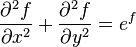
In differential geometry, Liouville's equation, named after Joseph Liouville, is the nonlinear partial differential equation satisfied by the conformal factor $f$ of a metric 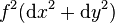$f^2(\mathrm{d}x^2 + \mathrm{d}y^2)$ on a surface of constant Gaussian curvature $K$ :

\Delta_0\log f = -K f^2,

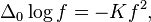
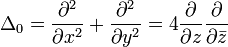
where $\Delta_0$ is the flat Laplace operator.

\Delta_0 = \frac{\partial^2}{\partial x^2} +\frac{\partial^2}{\partial y^2} = 4 \frac{\partial}{\partial z} \frac{\partial}{\partial \bar z}

Liouville's equation appears in the study of isothermal coordinates in differential geometry: the independent variables $x,y$ are the coordinates, while $f$ can be described as the conformal factor with respect to the flat metric. Occasionally it is the square $f^2$ that is referred to as the conformal factor, instead of $f$ itself.

Liouville's equation was also taken as an example by David Hilbert in the formulation of his nineteenth problem.^[1]

Other common forms of Liouville's equation

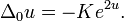
By using the change of variables " $\log \,f = u$ ", another commonly found form of Liouville's equation is obtained:

\Delta_0 u = - K e^{2u}.

Other two forms of the equation, commonly found in the literature,^[2] are obtained by using the slight variant " $2\log \,f = u$ " of the previous change of variables and Wirtinger calculus:^[3]

\Delta_0 u = - 2K e^{u}\quad\Longleftrightarrow\quad \frac{\partial^2 u}{{\partial z}{\partial \bar z}} = - \frac{K}{2} e^{u}.

Note that it is exactly in the first one of the preceding two forms that Liouville's equation was cited by David Hilbert in the formulation of his nineteenth problem.^[1]^[4]

A formulation using the Laplace-Beltrami operator

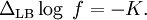
In a more invariant fashion, the equation can be written in terms of the intrinsic Laplace-Beltrami operator

\Delta_{\mathrm{LB}} = \frac{1}{f^2} \Delta_0

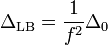
as follows:

\Delta_{\mathrm{LB}}\log\; f = -K.

Properties

Relation to Gauss–Codazzi equations

Liouville's equation is a consequence of the Gauss–Codazzi equations when the metric is written in isothermal coordinates.

General solution of the equation

In a simply connected domain $\Omega$ , the general solution of Liouville's equation can be found by using Wirtinger calculus.^[5] Its form is given by

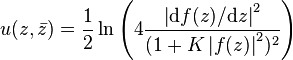
u(z,\bar z) = \frac{1}{2} \ln \left( 4 \frac{ \left|{\mathrm{d} f(z)}/{\mathrm{d} z}\right|^2 }{ ( 1+K \left|f(z)\right|^2)^2 } \right)

where $f(z)$ is any meromorphic function such that

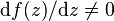${\mathrm{d} f(z)}/{\mathrm{d} z}\neq 0$ for every $z \in \Omega$ .^[5]
$f(z)$ has at most simple poles in $\Omega$ .^[5]

Application

Liouville's equation can be used to prove the following classification results for surfaces:

Theorem.^[6] A surface in the Euclidean 3-space with metric 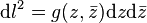$\mathrm{d}l^2 = g(z,{\bar z}){\mathrm{d}z}{\mathrm{d} \bar z}$ , and with constant scalar curvature $K$ is locally isometric to:

the sphere if $K > 0$ ;
the Euclidean plane if $K = 0$ ;
the Lobachevskian plane if $K < 0$ .

Notes

↑ 1.0 1.1 See (Hilbert 1900, p. 288): Hilbert does not cite explicitly Joseph Liouville.
↑ See (Dubrovin, Novikov & Fomenko 1992, p. 118) and (Henrici, p. 294).
↑ See (Henrici, pp. 287–294).
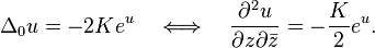
↑ Hilbert assumes $K = -1/2$ , therefore the equation appears as the following semilinear elliptic equation:
$\frac{\partial^2 f}{\partial x^2} + \frac{\partial^2 f}{\partial y^2} = e^f$
↑ 5.0 5.1 5.2 See (Henrici, p. 294).
↑ See (Dubrovin, Novikov & Fomenko 1992, pp. 118–120).

References

Dubrovin, B. A.; Novikov, S. P.; Fomenko, A. T. (1992) [1984], Modern Geometry–Methods and Applications. Part I. The Geometry of Surfaces, Transformation Groups, and Fields, Graduate Studies in Mathematics 93 (2nd ed.), Berlin–Heidelberg–New York: Springer Verlag, pp. xv+468, ISBN 3-540-97663-9, MR 0736837, Zbl 0751.53001
Henrici, Peter (1993) [1986], Applied and Computational Complex Analysis Volume 3, Wiley Classics Library (Reprint ed.), New York - Chichester - Brisbane - Toronto - Singapore: John Wiley & Sons, pp. X+637, ISBN 0-471-58986-1, MR 0822470, Zbl 1107.30300 .
Hilbert, David (1900), "Mathematische Probleme", Nachrichten von der Königlichen Gesellschaft der Wissenschaften zu Göttingen, Mathematisch-Physikalische Klasse (in German) (3): 253–297, JFM 31.0068.03 , translated in English by Mary Frances Winston Newson as Hilbert, David (1902), "Mathematical Problems", Bulletin of the American Mathematical Society 8 (10): 437–479, doi:10.1090/S0002-9904-1902-00923-3, JFM 33.0976.07, MR 1557926 .