Linear-fractional programming
In mathematical optimization, linear-fractional programming (LFP) is a generalization of linear programming (LP). Whereas the objective function in a linear program is a linear function, the objective function in a linear-fractional program is a ratio of two linear functions. A linear program can be regarded as a special case of a linear-fractional program in which the denominator is the constant function one.
Relation to linear programming
Both linear programming and linear-fractional programming represent optimization problems using linear equations and linear inequalities, which for each problem-instance define a feasible set. Fractional linear programs have a richer set of objective functions. Informally, linear programming computes a policy delivering the best outcome, such as maximum profit or lowest cost. In contrast, a linear-fractional programming is used to achieve the highest ratio of outcome to cost, the ratio representing the highest efficiency. For example, in the context of LP we maximize the objective function profit = income − cost and might obtain maximal profit of $100 (= $1100 of income − $1000 of cost). Thus, in LP we have an efficiency of $100/$1000 = 0.1. Using LFP we might obtain an efficiency of $10/$50 = 0.2 with a profit of only $10, which requires only $50 of investment however.
Definition
Formally, a linear-fractional program is defined as the problem of maximizing (or minimizing) a ratio of affine functions over a polyhedron,
where  represents the vector of variables to be determined,
  and
and  are vectors of (known) coefficients,
  is a (known) matrix of coefficients and
  are constants. The constraints have to restrict the feasible region to
  , i.e. the region on which the denominator is positive.[1][2] Alternatively, the denominator of the objective function has to be strictly negative in the entire feasible region.
Transformation to a linear program
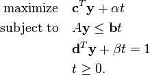
Under the assumption that the feasible region is non-empty and bounded, the Charnes-Cooper transformation[1]

translates the linear-fractional program above to the equivalent linear program:

Duality
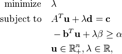
Let the dual variables associated with the constraints  and
and  be denoted by
  and
and  , respectively. Then the dual of the LFP above is [3][4]
which is an LP and which coincides with the dual of the equivalent linear program resulting from the Charnes-Cooper transformation.
Properties of and algorithms for linear-fractional programs
The objective function in a linear-fractional problem is both quasiconcave and quasiconvex (hence quasilinear) with a monotone property, pseudoconvexity, which is a stronger property than quasiconvexity. A linear-fractional objective function is both pseudoconvex and pseudoconcave, hence pseudolinear. Since an LFP can be transformed to an LP, it can be solved using any LP solution method, such as the simplex algorithm (of George B. Dantzig),[5][6][7][8] the criss-cross algorithm,[9] or interior-point methods.
Notes
- ↑ 1.0 1.1 Charnes, A.; Cooper, W. W. (1962). "Programming with Linear Fractional Functionals". Naval Research Logistics Quarterly 9: 181–196. doi:10.1002/nav.3800090303. MR 152370.
- ↑ Boyd, Stephen P.; Vandenberghe, Lieven (2004). Convex Optimization (pdf). Cambridge University Press. p. 151. ISBN 978-0-521-83378-3. Retrieved October 15, 2011.
- ↑ Schaible, Siegfried (1974). "Parameter-free Convex Equivalent and Dual Programs". Zeitschrift für Operations Research 18 (5): 187–196. doi:10.1007/BF02026600. MR 351464.
- ↑ Schaible, Siegfried (1976). "Fractional programming I: Duality". Management Science 22 (8): 858–867. doi:10.1287/mnsc.22.8.858. JSTOR 2630017. MR 421679.
- ↑ Chapter five: Craven, B. D. (1988). Fractional programming. Sigma Series in Applied Mathematics 4. Berlin: Heldermann Verlag. p. 145. ISBN 3-88538-404-3. MR 949209.
- ↑ Kruk, Serge; Wolkowicz, Henry (1999). "Pseudolinear programming". SIAM Review 41 (4): 795–805. doi:10.1137/S0036144598335259. JSTOR 2653207. MR 1723002.
- ↑ Mathis, Frank H.; Mathis, Lenora Jane (1995). "A nonlinear programming algorithm for hospital management". SIAM Review 37 (2): 230–234. doi:10.1137/1037046. JSTOR 2132826. MR 1343214.
- ↑ Murty (1983, Chapter 3.20 (pp. 160–164) and pp. 168 and 179)
- ↑ Illés, Tibor; Szirmai, Ákos; Terlaky, Tamás (1999). "The finite criss-cross method for hyperbolic programming". European Journal of Operational Research 114 (1): 198–214. doi:10.1016/S0377-2217(98)00049-6. Zbl 0953.90055. Postscript preprint.
References
- Craven, B. D. (1988). Fractional programming. Sigma Series in Applied Mathematics 4. Berlin: Heldermann Verlag. p. 145. ISBN 3-88538-404-3. MR 949209.
- Illés, Tibor; Szirmai, Ákos; Terlaky, Tamás (1999). "The finite criss-cross method for hyperbolic programming". European Journal of Operational Research 114 (1): 198–214. doi:10.1016/S0377-2217(98)00049-6. Zbl 0953.90055. Postscript preprint.
- Kruk, Serge; Wolkowicz, Henry (1999). "Pseudolinear programming". SIAM Review 41 (4): 795–805. doi:10.1137/S0036144598335259. JSTOR 2653207. MR 1723002.
- Mathis, Frank H.; Mathis, Lenora Jane (1995). "A nonlinear programming algorithm for hospital management". SIAM Review 37 (2): 230–234. doi:10.1137/1037046. JSTOR 2132826. MR 1343214.
- Murty, Katta G. (1983). "3.10 Fractional programming (pp. 160–164)". Linear programming. New York: John Wiley & Sons, Inc. pp. xix+482. ISBN 0-471-09725-X. MR 720547.
Further reading
- Bajalinov, E. B. (2003). Linear-Fractional Programming: Theory, Methods, Applications and Software. Boston: Kluwer Academic Publishers.
- Barros, Ana Isabel (1998). Discrete and fractional programming techniques for location models. Combinatorial Optimization 3. Dordrecht: Kluwer Academic Publishers. pp. xviii+178. ISBN 0-7923-5002-2. MR 1626973.
- Martos, Béla (1975). Nonlinear programming: Theory and methods. Amsterdam-Oxford: North-Holland Publishing Co. p. 279. ISBN 0-7204-2817-3. MR 496692.
- Schaible, S. (1995). "Fractional programming". In Reiner Horst and Panos M. Pardalos. Handbook of global optimization. Nonconvex optimization and its applications 2. Dordrecht: Kluwer Academic Publishers. pp. 495–608. ISBN 0-7923-3120-6. MR 1377091.
- Stancu-Minasian, I. M. (1997). Fractional programming: Theory, methods and applications. Mathematics and its applications 409. Translated by Victor Giurgiutiu from the 1992 Romanian. Dordrecht: Kluwer Academic Publishers Group. pp. viii+418. ISBN 0-7923-4580-0. MR 1472981.
Software
- WinGULF – educational interactive linear and linear-fractional programming solver with a lot of special options (pivoting, pricing, branching variables, etc.)
- JOptimizer – Java convex optimization library (open source)

