Lindhard theory
Lindhard theory[1][2] is a method of calculating the effects of electric field screening by electrons in a solid. It is based on quantum mechanics (first-order perturbation theory) and the random phase approximation.
Thomas–Fermi screening can be derived as a special case of the more general Lindhard formula. In particular, Thomas–Fermi screening is the limit of the Lindhard formula when the wavevector (the reciprocal of the length-scale of interest) is much smaller than the fermi wavevector, i.e. the long-distance limit.[2]
This article uses cgs-Gaussian units.
Formula
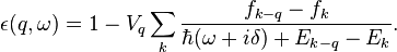
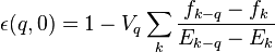
Lindhard formula for the longitudinal dielectric function is given by
Here,  is
is  and
and  is the carrier distribution function which is the Fermi–Dirac distribution function (see also Fermi–Dirac statistics) for electrons in thermodynamic equilibrium.
However this Lindhard formula is valid also for nonequilibrium distribution functions.
is the carrier distribution function which is the Fermi–Dirac distribution function (see also Fermi–Dirac statistics) for electrons in thermodynamic equilibrium.
However this Lindhard formula is valid also for nonequilibrium distribution functions.
Analysis of the Lindhard formula
For understanding the Lindhard formula, let's consider some limiting cases in 3 dimensions and 2 dimensions. 1 dimension case is also considered in other way.
Three dimensions
Long wave-length limit
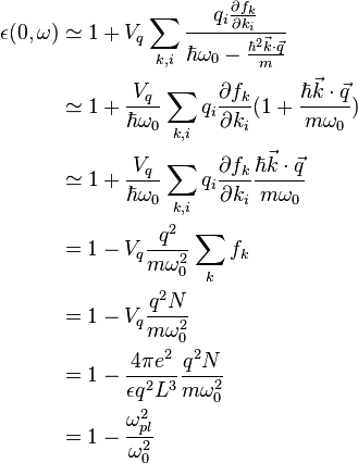
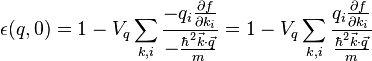
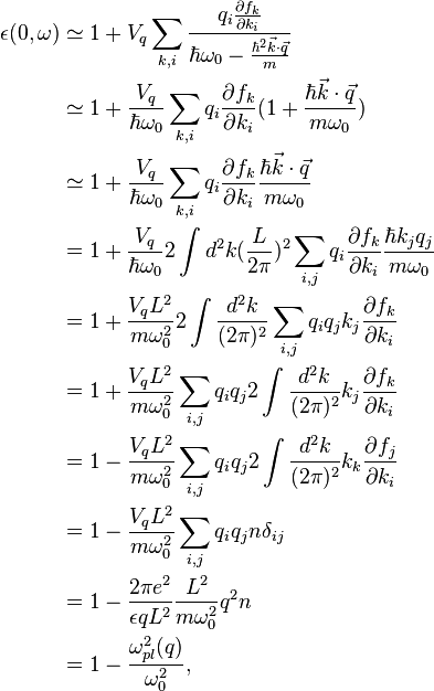
First, consider the long wavelength limit ( ).
).
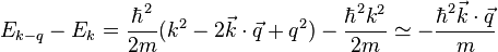
For denominator of Lindhard formula,
-
 ,
,
and for numerator of Lindhard formula,
-
 .
.
Inserting these to Lindhard formula and taking  limit, we obtain
-
 ,
,
where we used  ,
,  and
and  .
.
(In SI units, replace the factor  by
by  .)
.)
This result is same as the classical dielectric function.
Static Limit
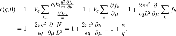
Second, consider the static limit ( ).
The Lindhard formula becomes
).
The Lindhard formula becomes
-
 .
.
Inserting above equalities for denominator and numerator to this, we obtain
-
 .
.
Assuming a thermal equilibrium Fermi–Dirac carrier distribution, we get
here, we used  and
and  .
.
Therefore,
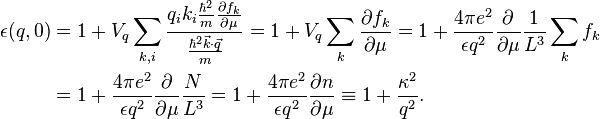
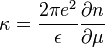
 is 3D screening wave number(3D inverse screening length) defined as
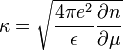 .
.
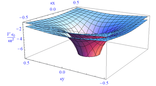
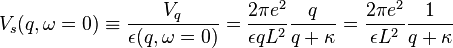
Then, the 3D statically screened Coulomb potential is given by
-
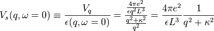 .
.
And Fourier transformation of this result gives
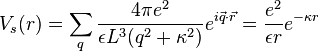
known as the Yukawa potential.
For a degenerating gas(T=0), Fermi energy is given by
-
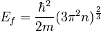 ,
,
So the density is
-
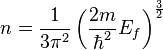 .
.
At T=0,  , so
, so  .
.
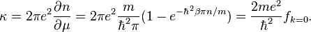
Inserting this to above 3D screening wave number equation, we get
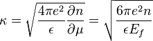 .
.
This is 3D Thomas–Fermi screening wave number.
For reference, Debye-Hückel screening describes the nondegenerate limit case.
The result is 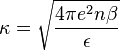 , 3D Debye-Hückel screening wave number.
Two dimensions
Long wave-length limit
First, consider the long wavelength limit ().
For denominator of Lindhard formula,
- ,
and for numerator of Lindhard formula,
-
 .
.
Inserting these to Lindhard formula and taking limit, we obtain
where we used  ,
,  and
and 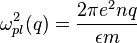 .
.
Static Limit
Second, consider the static limit ().
The Lindhard formula becomes
- .
Inserting above equalities for denominator and numerator to this, we obtain
- .
Assuming a thermal equilibrium Fermi–Dirac carrier distribution, we get
here, we used and .
Therefore,
is 2D screening wave number(2D inverse screening length) defined as
 .
.
Then, the 2D statically screened Coulomb potential is given by
-
 .
.
It is known that the chemical potential of the 2-dimensional Fermi gas is given by
-
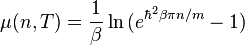 ,
,
and 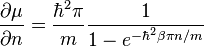 .
.
So, the 2D screening wave number is
Note that this result is independent of n.
One Dimension
This time, let's consider some generalized case for lowering the dimension. The lower the dimensions is, the weaker the screening effect is. In lower dimension, some of the field lines pass through the barrier material wherein the screening has no effect. For 1-dimensional case, we can guess that the screening effects only on the field lines which are very close to the wire axis.
Experiment
In real experiment, we should also take the 3D bulk screening effect into account even though we deal with 1D case like the single filament.
D. Davis applied the Thomas–Fermi screening to an electron gas confined to a filament and a coaxial cylinder.
For K2Pt(CN)4Cl0.32·2.6H20, it was found that the potential within the region between the filament and cylinder varies as
 and its effective screening length is about 10 times that of metallic platinum.
See also
- Electric field screening
References
- Haug, Hartmut; W. Koch, Stephan (2004). Quantum Theory of the Optical and Electronic Properties of Semiconductors (4th ed.). World Scientific Publishing Co. Pte. Ltd. ISBN 981-238-609-2.
- D. Davis Thomas-fermi screening in one dimension, Phys. Rev. B, 7(1), 129, (1973)