Lindblad equation

In quantum mechanics, Kossakowski–Lindblad equation (after Andrzej Kossakowski and Göran Lindblad) or master equation in Lindblad form is the most general type of Markovian and time-homogeneous master equation describing non-unitary evolution of the density matrix $ρ$ that is trace-preserving and completely positive for any initial condition.

Lindblad master equation for an $N$ -dimensional system's reduced density matrix $ρ$ can be written:

\dot\rho=-{i\over\hbar}[H,\rho]+\sum_{n,m = 1}^{N^2-1} h_{n,m}\left(L_n\rho L_m^\dagger-\frac{1}{2}\left(\rho L_m^\dagger L_n + L_m^\dagger L_n\rho\right)\right)

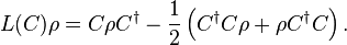
where $H$ is a (Hermitian) Hamiltonian part, the $L m$ are an arbitrary linear basis of the operators on the system's Hilbert space, and the $h n,m$ are constants which determine the dynamics. The coefficient matrix $h = (h n,m)$ must be positive to ensure that the equation is trace-preserving and completely positive. The summation only runs to $N 2 - 1$ because we have taken $L N 2$ to be proportional to the identity operator, in which case the summand vanishes. Our convention implies that the $L m$ are traceless for $m < N 2$ . The terms in the summation where $m = n$ can be described in terms of the Lindblad superoperator,

L(C)\rho=C\rho C^\dagger -\frac{1}{2}\left(C^\dagger C \rho +\rho C^\dagger C\right).

If the $h m,n$ terms are all zero, then this is quantum Liouville equation (for a closed system), which is the quantum analog of the classical Liouville equation. A related equation describes the time evolution of the expectation values of observables, it is given by the Ehrenfest theorem.

Note that $H$ is not necessarily equal to the self-Hamiltonian of the system. It may also incorporate effective unitary dynamics arising from the system-environment interaction.

Lindblad equations is also called the following equations for quantum observables:

\frac d{dt} A = -\frac 1{i\hbar} [H, A] + \frac 1{2\hbar} \sum^\infty_{k=1} \big(V^\dagger_k [A, V_k] + [V^\dagger_k, A] V_k \big),

where $A$ is a quantum observable.

Diagonalization

Since the matrix $h = (h n,m)$ is positive, it can be diagonalized with a unitary transformation $u$ :

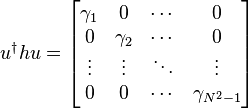
u^\dagger h u = \begin{bmatrix} \gamma_1 & 0 & \cdots & 0 \\ 0 & \gamma_2 & \cdots & 0 \\ \vdots & \vdots & \ddots & \vdots \\ 0 & 0 & \cdots & \gamma_{N^2-1} \end{bmatrix}

where the eigenvalues $γ i$ are non-negative. If we define another orthonormal operator basis

A_i = \sum_{j = 1}^{N^2-1} u_{j,i} L_j

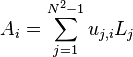
we can rewrite Lindblad equation in diagonal form

\dot\rho=-{i\over\hbar}[H,\rho]+\sum_{i = 1}^{N^2-1} \gamma_i\left(A_i\rho A_i^\dagger -\frac{1}{2} \rho A_i^\dagger A_i -\frac{1}{2} A_i^\dagger A_i \rho \right).

This equation is invariant under a unitary transformation of Lindblad operators and constants,

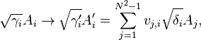
\sqrt{\gamma_i} A_i \to \sqrt{\gamma_i'} A_i' = \sum_{j = 1}^{N^2-1} v_{j,i} \sqrt{\delta_i} A_j ,

and also under the inhomogeneous transformation

A_i \to A_i' = A_i + a_i,

H \to H' = H + \frac{1}{2i} \sum_{j=1}^{N^2-1} \gamma_j \left (a_j^* A_j - a_j A_J^\dagger \right ).

However, the first transformation destroys the orthonormality of the operators $A i$ (unless all the $γ i$ are equal) and the second transformation destroys the tracelessness. Therefore, up to degeneracies among the $γ i$ , the $A i$ of the diagonal form of the Lindblad equation are uniquely determined by the dynamics so long as we require them to be orthonormal and traceless.

Harmonic oscillator example

The most common Lindblad equation is that describing the damping of a quantum harmonic oscillator, it has

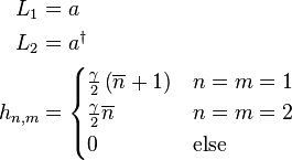
\begin{align} L_1 &= a \\ L_2 &= a^{\dagger} \\ h_{n,m} &= \begin{cases} \tfrac{\gamma}{2} \left (\overline{n}+1 \right ) & n=m=1 \\ \tfrac{\gamma}{2} \overline{n} & n=m=2 \\ 0 & \text{else} \end{cases} \end{align}

Here $\overline{n}$ is the mean number of excitations in the reservoir damping the oscillator and $γ$ is the decay rate. Additional Lindblad operators can be included to model various forms of dephasing and vibrational relaxation. These methods have been incorporated into grid-based density matrix propagation methods.

References

Kossakowski, A. (1972). "On quantum statistical mechanics of non-Hamiltonian systems". Rep. Math. Phys. 3 (4): 247. Bibcode:1972RpMP....3..247K. doi:10.1016/0034-4877(72)90010-9.
Lindblad, G. (1976). "On the generators of quantum dynamical semigroups". Commun. Math. Phys. 48 (2): 119. Bibcode:1976CMaPh..48..119L. doi:10.1007/BF01608499.
Gorini, V.; Kossakowski, A.; Sudarshan, E.C.G. (1976). "Completely positive semigroups of N-level systems". J. Math. Phys. 17 (5): 821. Bibcode:1976JMP....17..821G. doi:10.1063/1.522979.
Banks, T.; Susskind, L.; Peskin, M.E. (1984). "Difficulties for the evolution of pure states into mixed states". Nuclear Physics B 244: 125–134. Bibcode:1984NuPhB.244..125B. doi:10.1016/0550-3213(84)90184-6.
Accardi, Luigi; Lu, Yun Gang; Volovich, I.V. (2002). Quantum Theory and Its Stochastic Limit. New York: Springer Verlag. ISBN 978-3-5404-1928-0.
Alicki, Robert; Lendi, Karl (1987). Quantum Dynamical Semigroups and Applications. Berlin: Springer Verlag. ISBN 978-0-3871-8276-6.
Attal, Stéphane; Joye, Alain; Pillet, Claude-Alain (2006). Open Quantum Systems II: The Markovian Approach. Springer. ISBN 978-3-5403-0992-5.
Breuer, Heinz-Peter; Petruccione, F. (2002). The Theory of Open Quantum Systems. Oxford University Press. ISBN 978-0-1985-2063-4.
Gardiner, C.W.; Zoller, Peter (2010). Quantum Noise. Springer Series in Synergetics (3rd ed.). Berlin Heidelberg: Springer-Verlag. ISBN 978-3-642-06094-6.
Ingarden, Roman S.; Kossakowski, A.; Ohya, M. (1997). Information Dynamics and Open Systems: Classical and Quantum Approach. New York: Springer Verlag. ISBN 978-0-7923-4473-5.
Lindblad, G. (1983). Non-Equilibrium Entropy and Irreversibility. Dordrecht: Delta Reidel. ISBN 1-4020-0320-X.
Tarasov, Vasily E. (2008). Quantum Mechanics of Non-Hamiltonian and Dissipative Systems. Amsterdam, Boston, London, New York: Elsevier Science. ISBN 978-0-0805-5971-1.

External links

The Lindblad master equation

Lindblad equation

Diagonalization

Harmonic oscillator example

See also

References

External links