Latent Dirichlet allocation
In natural language processing, latent Dirichlet allocation (LDA) is a generative model that allows sets of observations to be explained by unobserved groups that explain why some parts of the data are similar. For example, if observations are words collected into documents, it posits that each document is a mixture of a small number of topics and that each word's creation is attributable to one of the document's topics. LDA is an example of a topic model and was first presented as a graphical model for topic discovery by David Blei, Andrew Ng, and Michael Jordan in 2003.[1]
Topics in LDA
In LDA, each document may be viewed as a mixture of various topics. This is similar to probabilistic latent semantic analysis (pLSA), except that in LDA the topic distribution is assumed to have a Dirichlet prior. In practice, this results in more reasonable mixtures of topics in a document. It has been noted, however, that the pLSA model is equivalent to the LDA model under a uniform Dirichlet prior distribution.[2]
For example, an LDA model might have topics that can be classified as CAT_related and DOG_related. A topic has probabilities of generating various words, such as milk, meow, and kitten, which can be classified and interpreted by the viewer as "CAT_related". Naturally, the word cat itself will have high probability given this topic. The DOG_related topic likewise has probabilities of generating each word: puppy, bark, and bone might have high probability. Words without special relevance, such as the (see function word), will have roughly even probability between classes (or can be placed into a separate category). A topic is not strongly defined, neither semantically nor epistemologically. It is identified on the basis of supervised labeling and (manual) pruning on the basis of their likelihood of co-occurrence. A lexical word may occur in several topics with a different probability, however, with a different typical set of neighboring words in each topic.
Each document is assumed to be characterized by a particular set of topics. This is akin to the standard bag of words model assumption, and makes the individual words exchangeable.
Model
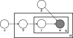
With plate notation, the dependencies among the many variables can be captured concisely. The boxes are “plates” representing replicates. The outer plate represents documents, while the inner plate represents the repeated choice of topics and words within a document. M denotes the number of documents, N the number of words in a document. Thus:
- α is the parameter of the Dirichlet prior on the per-document topic distributions,
- β is the parameter of the Dirichlet prior on the per-topic word distribution,
-
 is the topic distribution for document i,
 -
 is the word distribution for topic k,
 -
 is the topic for the jth word in document i, and
 -
 is the specific word.
The are the only observable variables, and the other variables are latent variables.
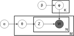
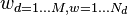
Mostly, the basic LDA model will be extended to a smoothed version to gain better results . The plate notation is shown on the right, where K denotes the number of topics considered in the model and:
-
 is a K*V (V is the dimension of the vocabulary) Markov matrix each row of which denotes the word distribution of a topic.
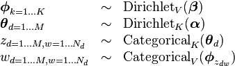
The generative process behind is that documents are represented as random mixtures over latent topics, where each topic is characterized by a distribution over words. LDA assumes the following generative process for a corpus  consisting of
  documents each of length
  :
:
1. Choose  , where
  and
and
 is the Dirichlet distribution for parameter
2. Choose  , where
3. For each of the word positions  , where
  , and
, and
- (a) Choose a topic
- (b) Choose a word
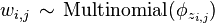 .
.
(Note that the Multinomial distribution here refers to the Multinomial with only one trial. It is formally equivalent to the categorical distribution.)
The lengths are treated as independent of all the other data generating variables ( and
and  ). The subscript is often dropped, as in the plate diagrams shown here.
Mathematical definition
A formal description of smoothed LDA is as follows:
| Variable | Type | Meaning |
|---|---|---|
 | integer | number of topics (e.g. 50) |
 | integer | number of words in the vocabulary (e.g. 50,000 or 1,000,000) |
| | integer | number of documents |
 | integer | number of words in document d |
 | integer | total number of words in all documents; sum of all  values, i.e. values, i.e.  |
 | positive real | prior weight of topic k in a document; usually the same for all topics; normally a number less than 1, e.g. 0.1, to prefer sparse topic distributions, i.e. few topics per document |
 | K-dimension vector of positive reals | collection of all  values, viewed as a single vector values, viewed as a single vector |
 | positive real | prior weight of word w in a topic; usually the same for all words; normally a number much less than 1, e.g. 0.001, to strongly prefer sparse word distributions, i.e. few words per topic |
 | V-dimension vector of positive reals | collection of all  values, viewed as a single vector values, viewed as a single vector |
 | probability (real number between 0 and 1) | probability of word w occurring in topic k |
 | V-dimension vector of probabilities, which must sum to 1 | distribution of words in topic k |
 | probability (real number between 0 and 1) | probability of topic k occurring in document d for any given word |
 | K-dimension vector of probabilities, which must sum to 1 | distribution of topics in document d |
 | integer between 1 and K | identity of topic of word w in document d |
 | N-dimension vector of integers between 1 and K | identity of topic of all words in all documents |
 | integer between 1 and V | identity of word w in document d |
 | N-dimension vector of integers between 1 and V | identity of all words in all documents |
We can then mathematically describe the random variables as follows:
Inference
Learning the various distributions (the set of topics, their associated word probabilities, the topic of each word, and the particular topic mixture of each document) is a problem of Bayesian inference. The original paper used a variational Bayes approximation of the posterior distribution;[1] alternative inference techniques use Gibbs sampling[3] and expectation propagation.[4]
Following is the derivation of the equations for collapsed Gibbs sampling, which means  s and
s and
 s will be integrated out. For simplicity, in this derivation the documents are all assumed to have the same length
  . The derivation is equally valid if the document lengths vary.
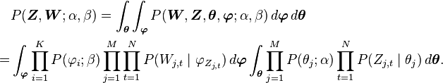
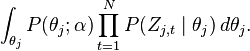
According to the model, the total probability of the model is:

where the bold-font variables denote the vector version of the
variables. First of all,  and
and
 need to be integrated out.
All the s are independent to each other
and the same to all the s. So we can treat each
and each separately. We now
focus only on the part.
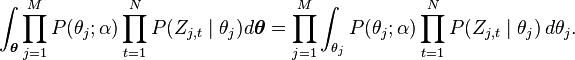
We can further focus on only one as the
following:
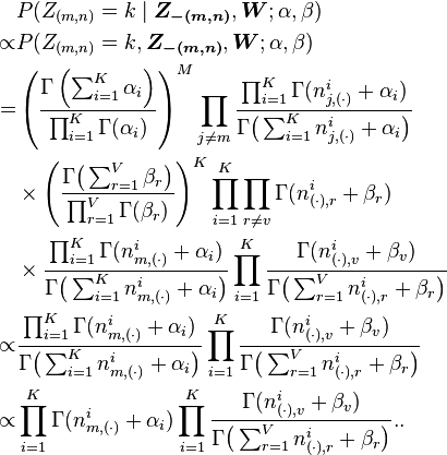
Actually, it is the hidden part of the model for the
 document. Now we replace the probabilities in
the above equation by the true distribution expression to write out
the explicit equation.
document. Now we replace the probabilities in
the above equation by the true distribution expression to write out
the explicit equation.

Let  be the number of word tokens in the
document with the same word symbol (the
be the number of word tokens in the
document with the same word symbol (the
 word in the vocabulary) assigned to the
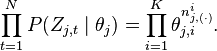
 topic. So, is three
dimensional. If any of the three dimensions is not limited to a specific value, we use a parenthesized point
topic. So, is three
dimensional. If any of the three dimensions is not limited to a specific value, we use a parenthesized point  to
denote. For example,
to
denote. For example,  denotes the number
of word tokens in the document assigned to the
topic. Thus, the right most part of the above
equation can be rewritten as:
denotes the number
of word tokens in the document assigned to the
topic. Thus, the right most part of the above
equation can be rewritten as:
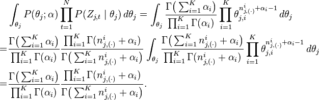
So the  integration formula can be changed to:
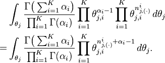
Clearly, the equation inside the integration has the same form as the Dirichlet distribution. According to the Dirichlet distribution,
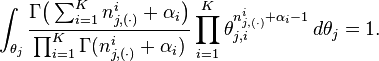
Thus,
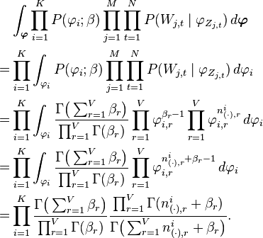
Now we turn our attentions to the
part. Actually, the derivation of the
part is very similar to the
part. Here we only list the steps
of the derivation:
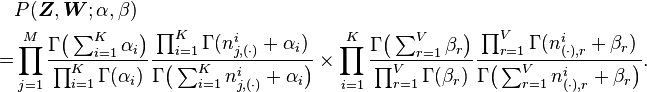
For clarity, here we write down the final equation with both
 and
integrated out:
and
integrated out:
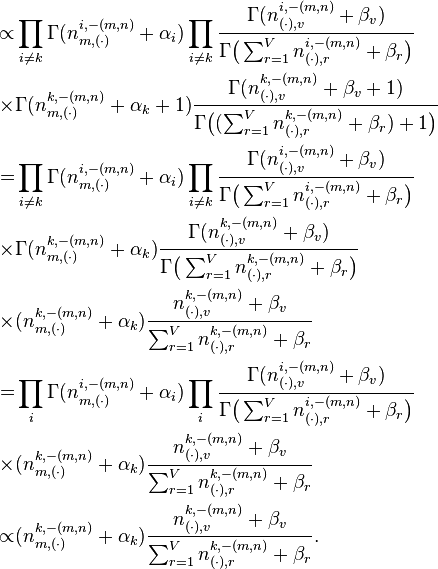
The goal of Gibbs Sampling here is to approximate the distribution of 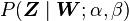 . Since
  is invariable for any of Z, Gibbs Sampling equations can be derived from
 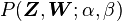 directly. The key point is to derive the following conditional probability:

where  denotes the
  hidden
variable of the
hidden
variable of the  word token in the
 document. And further we assume that the word
symbol of it is the
document. And further we assume that the word
symbol of it is the  word in the vocabulary.
 denotes all the s
but . Note that Gibbs Sampling needs only to
sample a value for , according to the above
probability, we do not need the exact value of
denotes all the s
but . Note that Gibbs Sampling needs only to
sample a value for , according to the above
probability, we do not need the exact value of
 but the ratios among the
probabilities that can take value. So, the
above equation can be simplified as:
but the ratios among the
probabilities that can take value. So, the
above equation can be simplified as:
Finally, let  be the same meaning as
but with the excluded.
The above equation can be further simplified leveraging the property
of gamma function. We first split the summation and then merge
it back to obtain a
be the same meaning as
but with the excluded.
The above equation can be further simplified leveraging the property
of gamma function. We first split the summation and then merge
it back to obtain a  -independent summation, which
could be dropped:
-independent summation, which
could be dropped:
Note that the same formula is derived in the article on the Dirichlet-multinomial distribution, as part of a more general discussion of integrating Dirichlet distribution priors out of a Bayesian network.
Applications, extensions and similar techniques
Topic modeling is a classic problem in information retrieval. Related models and techniques are, among others, latent semantic indexing, independent component analysis, probabilistic latent semantic indexing, non-negative matrix factorization, and Gamma-Poisson distribution.
The LDA model is highly modular and can therefore be easily extended. The main field of interest is modeling relations between topics. This is achieved by using another distribution on the simplex instead of the Dirichlet. The Correlated Topic Model[5] follows this approach, inducing a correlation structure between topics by using the logistic normal distribution instead of the Dirichlet. Another extension is the hierarchical LDA (hLDA),[6] where topics are joined together in a hierarchy by using the nested Chinese restaurant process. LDA can also be extended to a corpus in which a document includes two types of information (e.g., words and names), as in the LDA-dual model.[7] Nonparametric extensions of LDA include the Hierarchical Dirichlet process mixture model, which allows the number of topics to be unbounded and learnt from data and the Nested Chinese Restaurant Process which allows topics to be arranged in a hierarchy whose structure is learnt from data.
As noted earlier, PLSA is similar to LDA. The LDA model is essentially the Bayesian version of PLSA model. The Bayesian formulation tends to perform better on small datasets because Bayesian methods can avoid overfitting the data. For very large datasets, the results of the two models tend to converge. One difference is that PLSA uses a variable  to represent a document in the training set. So in PLSA, when presented with a document the model hasn't seen before, we fix
  —the probability of words under topics—to be that learned from the training set and use the same EM algorithm to infer
  —the topic distribution under . Blei argues that this step is cheating because you are essentially refitting the model to the new data.
Variations on LDA have been used to automatically put natural images into categories, such as "bedroom" or "forest", by treating an image as a document, and small patches of the image as words;[8] one of the variations is called Spatial Latent Dirichlet Allocation.[9]
Recently, LDA has been also applied to bioinformatics context.[10]
See also
- Pachinko allocation
- tf-idf
Notes
- ↑ 1.0 1.1 Blei, David M.; Ng, Andrew Y.; Jordan, Michael I (January 2003). Lafferty, John, ed. "Latent Dirichlet allocation". Journal of Machine Learning Research 3 (4–5): pp. 993–1022. doi:10.1162/jmlr.2003.3.4-5.993.
- ↑ Girolami, Mark; Kaban, A. (2003). On an Equivalence between PLSI and LDA. Proceedings of SIGIR 2003. New York: Association for Computing Machinery. ISBN 1-58113-646-3.
- ↑ Griffiths, Thomas L.; Steyvers, Mark (April 6, 2004). "Finding scientific topics". Proceedings of the National Academy of Sciences 101 (Suppl. 1): 5228–5235. doi:10.1073/pnas.0307752101. PMC 387300. PMID 14872004.
- ↑ Minka, Thomas; Lafferty, John (2002). Expectation-propagation for the generative aspect model. Proceedings of the 18th Conference on Uncertainty in Artificial Intelligence. San Francisco, CA: Morgan Kaufmann. ISBN 1-55860-897-4.
- ↑ Blei, David M.; Lafferty, John D. (2006). "Correlated topic models". Advances in Neural Information Processing Systems 18.
- ↑ Blei, David M.; Jordan, Michael I.; Griffiths, Thomas L.; Tenenbaum, Joshua B (2004). Hierarchical Topic Models and the Nested Chinese Restaurant Process. Advances in Neural Information Processing Systems 16: Proceedings of the 2003 Conference. MIT Press. ISBN 0-262-20152-6.
- ↑ Shu, Liangcai; Long, Bo; Meng, Weiyi (2009). A Latent Topic Model for Complete Entity Resolution. 25th IEEE International Conference on Data Engineering (ICDE 2009).
- ↑ Li, Fei-Fei; Perona, Pietro. "A Bayesian Hierarchical Model for Learning Natural Scene Categories". Proceedings of the 2005 IEEE Computer Society Conference on Computer Vision and Pattern Recognition (CVPR'05) 2: 524–531.
- ↑ Wang, Xiaogang; Grimson, Eric (2007). "Spatial Latent Dirichlet Allocation". Proceedings of Neural Information Processing Systems Conference (NIPS).
- ↑ "Latent Dirichlet Allocation based on Gibbs Sampling for gene function prediction"
External links
- Extremely useful lecture for understanding LDA: LDA and Topic Modelling Video Lecture by David Blei or same lecture on YouTube
- D. Mimno's LDA Bibliography An exhaustive list of LDA-related resources (incl. papers and some implementations)
- Gensim, a Python+NumPy implementation of online LDA for inputs larger than the available RAM.
- topicmodels and lda are two R packages for LDA analysis.
- "Text Mining with R" including LDA methods, video presentation to the October 2011 meeting of the Los Angeles R users group
- MALLET Open source Java-based package from the University of Massachusetts-Amherst for topic modeling with LDA, also has an independently developed GUI, the Topic Modeling Tool
- LDA in Mahout implementation of LDA using MapReduce on the Hadoop platform
- Latent Dirichlet Allocation (LDA) Tutorial for the Infer.NET Machine Computing Framework Microsoft Research C# Machine Learning Framework
| ||||||||||||||||||||||||||||||||||