Laplacian matrix

In the mathematical field of graph theory, the Laplacian matrix, sometimes called admittance matrix, Kirchhoff matrix or discrete Laplacian, is a matrix representation of a graph. Together with Kirchhoff's theorem, it can be used to calculate the number of spanning trees for a given graph. The Laplacian matrix can be used to find many other properties of the graph. Cheeger's inequality from Riemannian geometry has a discrete analogue involving the Laplacian matrix; this is perhaps the most important theorem in spectral graph theory and one of the most useful facts in algorithmic applications. It approximates the sparsest cut of a graph through the second eigenvalue of its Laplacian.

Definition

Given a simple graph G with n vertices, its Laplacian matrix $L:=(\ell_{i,j})_{n \times n}$ is defined as:^[1]

L = D - A,

where D is the degree matrix and A is the adjacency matrix of the graph. In the case of directed graphs, either the indegree or outdegree might be used, depending on the application.

From the definition it follows that:

\ell_{i,j}:= \begin{cases} \deg(v_i) & \mbox{if}\ i = j \\ -1 & \mbox{if}\ i \neq j\ \mbox{and}\ v_i \mbox{ is adjacent to } v_j \\ 0 & \mbox{otherwise} \end{cases}

where deg(v_i) is degree of the vertex i.

The normalized Laplacian matrix is defined as:^[1]

\mathcal{L} := D^{-1/2}LD^{-1/2}= I - D^{-1/2}AD^{-1/2} = (\tilde{\ell}_{ij})

where:

\tilde{\ell}_{i,j}:= \begin{cases} 1 & \mbox{if}\ i = j\ \mbox{and}\ \deg(v_i) \neq 0\\ -\frac{1}{\sqrt{\deg(v_i)\deg(v_j)}} & \mbox{if}\ i \neq j\ \mbox{and}\ v_i \mbox{ is adjacent to } v_j \\ 0 & \mbox{otherwise}. \end{cases}

Example

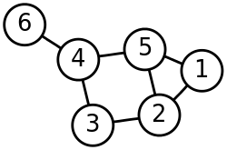
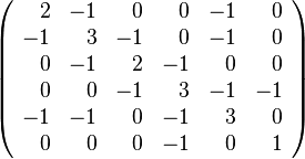
Here is a simple example of a labeled graph and its Laplacian matrix.

Labeled graph	Degree matrix	Adjacency matrix	Laplacian matrix
	$\left(\begin{array}{rrrrrr} 2 & 0 & 0 & 0 & 0 & 0\\ 0 & 3 & 0 & 0 & 0 & 0\\ 0 & 0 & 2 & 0 & 0 & 0\\ 0 & 0 & 0 & 3 & 0 & 0\\ 0 & 0 & 0 & 0 & 3 & 0\\ 0 & 0 & 0 & 0 & 0 & 1\\ \end{array}\right)$	$\left(\begin{array}{rrrrrr} 0 & 1 & 0 & 0 & 1 & 0\\ 1 & 0 & 1 & 0 & 1 & 0\\ 0 & 1 & 0 & 1 & 0 & 0\\ 0 & 0 & 1 & 0 & 1 & 1\\ 1 & 1 & 0 & 1 & 0 & 0\\ 0 & 0 & 0 & 1 & 0 & 0\\ \end{array}\right)$	$\left(\begin{array}{rrrrrr} 2 & -1 & 0 & 0 & -1 & 0\\ -1 & 3 & -1 & 0 & -1 & 0\\ 0 & -1 & 2 & -1 & 0 & 0\\ 0 & 0 & -1 & 3 & -1 & -1\\ -1 & -1 & 0 & -1 & 3 & 0\\ 0 & 0 & 0 & -1 & 0 & 1\\ \end{array}\right)$

Properties

For an (undirected) graph G and its Laplacian matrix L with eigenvalues $\lambda_0 \le \lambda_1 \le \cdots \le \lambda_{n-1}$ :

L is symmetric.
L is positive-semidefinite (that is $\lambda_i \ge 0$ for all i). This is verified in the incidence matrix section (below). This can also be seen from the fact that the Laplacian is symmetric and diagonally dominant.
L is an M-matrix (its off-diagonal entries are nonpositive, yet the real parts of its eigenvalues are nonnegative).
Every row sum and column sum of L is zero. Indeed, in the sum, the degree of the vertex is summed with a "-1" for each neighbor.
In consequence, $\lambda_0=0$ , because the vector $\mathbf{v}_0=(1,1,\dots,1)$ satisfies $L \mathbf{v}_0 = \mathbf{0} .$
The number of times 0 appears as an eigenvalue in the Laplacian is the number of connected components in the graph.
The smallest non-zero eigenvalue of L is called the spectral gap.
The second smallest eigenvalue of L is the algebraic connectivity (or Fiedler value) of G.
The Laplacian is an operator on the n-dimensional vector space of functions f : V → $\mathbb{R}$ , where V is the vertex set of G, and n = |V|.
When G is k-regular, the normalized Laplacian is: $\mathcal{L} = \tfrac{1}{k} L = I - \tfrac{1}{k} A$ , where A is the adjacency matrix and I is an identity matrix.
For a graph with multiple connected components, L is a block diagonal matrix, where each block is the respective Laplacian matrix for each component, possibly after reordering the vertices (i.e. L is permutation-similar to a block diagonal matrix).

Incidence matrix

Define an $|e|$ x $|v|$ oriented incidence matrix M with element M_ev for edge e (connecting vertex i and j, with i > j) and vertex v given by

M_{ev} = \left\{ \begin{array}{rl}1, & \text{if}\,v=i\\-1, & \text{if}\,v=j\\0, & \text{otherwise}.\end{array}\right.

Then the Laplacian matrix L satisfies

L = M^\text{T} M\,,

where $M^\text{T}$ is the matrix transpose of M.

Now consider an eigendecomposition of $L$ , with unit-norm eigenvectors $\mathbf{v}_i$ and corresponding eigenvalues $\lambda_i$ :

\begin{align} \lambda_i & = \mathbf{v}_i^T L \mathbf{v}_i \\ & = \mathbf{v}_i^T M^T M \mathbf{v}_i \\ & = (M \mathbf{v}_i)^T (M \mathbf{v}_i). \\ \end{align}

Because $\lambda_i$ can be written as the inner product of the vector $M \mathbf{v}_i$ with itself, this shows that $\lambda_i \ge 0$ and so the eigenvalues of $L$ are all non-negative.

Deformed Laplacian

The deformed Laplacian is commonly defined as

\Delta(s)=I-sA+s^2(D-I)

where I is the unit matrix, A is the adjacency matrix, and D is the degree matrix, and s is a (complex-valued) number. Note that the standard Laplacian is just $\Delta(1)$ .^[2]

Symmetric normalized Laplacian

The (symmetric) normalized Laplacian is defined as

\mathcal{L}:= D^{-1/2} L D^{-1/2} = I-D^{-1/2}AD^{-1/2}

where L is the Laplacian, A is the adjacency matrix and D is the degree matrix. Since the degree matrix D is diagonal and positive, its reciprocal square root $D^{-1/2}$ is just the diagonal matrix whose diagonal entries are the reciprocals of the positive square roots of the diagonal entries of D. The symmetric normalized Laplacian is a symmetric matrix.

One has: $\mathcal{L} = S S^{*}$ , where S is the matrix whose rows are indexed by the vertices and whose columns are indexed by the edges of G such that each column corresponding to an edge e = {u, v} has an entry $\frac{1}{\sqrt d_{u}}$ in the row corresponding to u, an entry $-\frac{1}{\sqrt d_{v}}$ in the row corresponding to v, and has 0 entries elsewhere. (Note: $S^{*}$ denotes the transpose of S).

All eigenvalues of the normalized Laplacian are real and non-negative. We can see this as follows. Since $\mathcal{L}$ is symmetric, its eigenvalues are real. They are also non-negative: consider an eigenvector g of $\mathcal{L}$ with eigenvalue λ and suppose $g = D^{1/2} f$ . (We can consider g and f as real functions on the vertices v.) Then:

\lambda \ {} = \ {} \frac{\langle g,\mathcal{L}g\rangle}{\langle g, g\rangle} \ {} = \ {} \frac{\langle g, D^{-1/2} L D^{-1/2} g\rangle}{\langle g,g\rangle} \ {} = \ {} \frac{\langle f, Lf\rangle}{\langle D^{1/2} f, D^{1/2} f\rangle} \ {} = \ {} \frac{\sum_{u\sim v}(f(u) - f(v) )^2}{\sum_{v} f(v)^2 d_{v}} \ > \ 0,

where we use the inner product $\langle f,g\rangle = \sum_{v} f(v)g(v)$ , a sum over all vertices v, and $\sum_{u\sim v}$ denotes the sum over all unordered pairs of adjacent vertices {u,v}. The quantity $\sum_{u,v}(f(u) - f(v) )^2$ is called the Dirichlet sum of f, whereas the expression $\frac{\langle g,\mathcal{L}g\rangle}{\langle g, g\rangle}$ is called the Rayleigh quotient of g.

Let 1 be the function which assumes the value 1 on each vertex. Then $D^{1/2} 1$ is an eigenfunction of $\mathcal{L}$ with eigenvalue 0.^[3]

In fact, the eigenvalues of the normalized Laplacian satisfy 0 = μ₀≤...≤ μ_n-1≤ 2. These eigenvalues (known as the spectrum of the normalized Laplacian) relate well to other graph invariants for general graphs.^[4]

Random walk normalized Laplacian

The random walk normalized Laplacian is defined as

T:=D^{-1}A

where A is the adjacency matrix and D is the degree matrix. Since the degree matrix D is diagonal, its inverse $D^{-1}$ is simply defined as a diagonal matrix, having diagonal entries which are the reciprocals of the corresponding positive diagonal entries of D. The name of this operator comes from the fact that, indeed, $T$ is the transition matrix of a standard random walk on the given graph.

One can check that

T=D^{-\frac12} \left(I-\mathcal{L}\right) D^{\frac12}

i.e., $T$ is similar to a scalar perturbation of the normalized Laplacian $\mathcal{L}$ . For this reason, even if $T$ is in general not hermitian, it has real eigenvalues. Indeed, its eigenvalues agree with those of $\mathcal{L}$ (which is hermitian), up to a mirroring in the point $1/2$ .

Graphs

As an aside about random walks on graphs, consider a simple undirected graph. Consider the probability that the walker is at the vertex i at time t, given the probability distribution that he was at vertex j at time t-1 (assuming a uniform chance of taking a step along any of the edges attached to a given vertex):

p_i(t) = \sum_j \frac{A_{ij}}{deg(v_j)} p_j(t-1),

or in matrix-vector notation:

p(t) = A D^{-1} p(t-1).

(Equilibrium, which sets in as $t\rightarrow \infty$ , is defined by $p = A D^{-1} p$ .)

We can rewrite this relation as

\begin{align} D^{-\frac12} p(t) & = \left[ D^{-\frac12} A D^{-\frac12} \right] D^{-\frac12} p(t-1). \end{align}

$A_{reduced} \equiv D^{-\frac12} A D^{-\frac12}$ is a symmetric matrix called the reduced adjacency matrix. So, taking steps on this random walk requires taking powers of $A_{reduced}$ , which is a simple operation because $A_{reduced}$ is symmetric.

Interpretation as the discrete Laplace operator

The Laplacian matrix can be interpreted as a matrix representation of a particular case of the discrete Laplace operator. Such an interpretation allows one, e.g., to generalise the Laplacian matrix to the case of graphs with an infinite number of vertices and edges, leading to a Laplacian matrix of an infinite size.

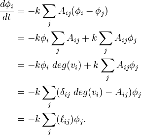
To expand upon this, we can "describe" the change of some element $\phi_i$ (with some constant k) as

\begin{align} \frac{d \phi_i}{d t} & = -k \sum_j A_{ij} (\phi_i - \phi_j) \\ & = -k \phi_i \sum_j A_{ij} + k \sum_j A_{ij} \phi_j \\ & = - k \phi_i \ deg(v_i) + k \sum_j A_{ij} \phi_j \\ & = - k \sum_j (\delta_{ij} \ deg(v_i) - A_{ij} ) \phi_j \\ & = -k \sum_j (\ell_{ij} ) \phi_j. \end{align}

In matrix-vector notation,

\begin{align} \frac{d \phi}{d t} & = -k(D-A)\phi \\ & = -k L \phi, \end{align}

which gives

\begin{align} \frac{d \phi}{d t} + kL\phi = 0. \end{align}

Notice that this equation takes the same form as the heat equation, where the matrix L is replacing the Laplacian operator $\nabla^2$ ; hence, the "graph Laplacian".

To find a solution to this differential equation, apply standard techniques for solving a first-order matrix differential equation. That is, write $\phi$ as a linear combination of eigenvectors $\mathbf{v}_i$ of L (so that $L\mathbf{v}_i = \lambda_i \mathbf{v}_i$ ), with time-dependent $\begin{align} \phi = \sum_i c_i \mathbf{v}_i. \end{align}$

Plugging into the original expression (note that we will use the fact that because L is a symmetric matrix, its unit-norm eigenvectors $\mathbf{v}_i$ are orthogonal):

\begin{align} \frac{d (\sum_i c_i \mathbf{v}_i)}{d t} + kL(\sum_i c_i \mathbf{v}_i) & = 0 \\ \sum_i \left[ \frac{d c_i}{d t} \mathbf{v}_i + k c_i L \mathbf{v}_i \right] & = \\ \sum_i \left[ \frac{d c_i}{d t} \mathbf{v}_i + k c_i \lambda_i \mathbf{v}_i \right] & = \\ \frac{d c_i}{d t} + k \lambda_i c_i & = 0, \\ \end{align}

whose solution is

\begin{align} c_i(t) = c_i(0) \exp(-k \lambda_i t). \end{align}

As shown before, the eigenvalues $\lambda_i$ of L are non-negative, showing that the solution to the diffusion equation approaches an equilibrium, because it only exponentially decays or remains constant. This also shows that given $\lambda_i$ and the initial condition $c_i(0)$ , the solution at any time t can be found.^[5]

To find $c_i(0)$ for each $i$ in terms of the overall initial condition $\phi(0)$ , simply project $\phi(0)$ onto the unit-norm eigenvectors $\mathbf{v}_i$ ;

$c_i(0) = \langle \phi(0), \mathbf{v}_i \rangle$ .

In the case of undirected graphs, this works because $L$ is symmetric, and by the spectral theorem, its eigenvectors are all orthogonal. So the projection onto the eigenvectors of $L$ is simply an orthogonal coordinate transformation of the initial condition to a set of coordinates which decay exponentially and independently of each other.

Equilibrium Behavior

To understand $\lim_{t \to \infty}\phi(t)$ , note that the only terms $c_i(t) = c_i(0) \exp(-k \lambda_i t)$ that remain are those where $\lambda_i = 0$ , since

$\lim_{t \to \infty} \exp(-k \lambda_i t) = \left\{ \begin{array}{rlr}0 & \text{if} &\lambda_i > 0 \\ 1 & \text{if} & \lambda_i = 0 \end{array} \right\}$

In other words, the equilibrium state of the system is determined completely by the kernel of $L$ . Since by definition, $\sum_{j}L_{ij} = 0$ , the vector $\mathbf{v}^1$ of all ones is in the kernel. Note also that if there are $k$ disjoint connected components in the graph, then this vector of all ones can be split into the sum of $k$ independent $\lambda = 0$ eigenvectors of ones and zeros, where each connected component corresponds to an eigenvector with ones at the elements in the connected component and zeros elsewhere.

The consequence of this is that for a given initial condition $c(0)$ for a graph with $N$ vertices

$\lim_{t \to \infty}\phi(t) = \langle c(0), \mathbf{v^1} \rangle \mathbf{v^1}$

where

$\mathbf{v^1} = \frac{1}{\sqrt{N}} [1, 1, ..., 1]$

For each element $\phi_j$ of $\phi$ , i.e. for each vertex $j$ in the graph, it can be rewritten as

$\lim_{t \to \infty}\phi_j(t) = \frac{1}{N} \sum_{i = 1}^N c_i(0)$ .

In other words, at steady state, the value of $\phi$ converges to the same value at each of the vertices of the graph, which is the average of the initial values at all of the vertices. Since this is the solution to the heat diffusion equation, this makes perfect sense intuitively. We expect that neighboring elements in the graph will exchange energy until that energy is spread out evenly throughout all of the elements that are connected to each other.

Example of the Operator on a Grid

This GIF shows the progression of diffusion, as solved by the graph laplacian technique. A graph is constructed over a grid, where each pixel in the graph is connected to its 8 bordering pixels. Values in the image then diffuse smoothly to their neighbors over time via these connections. This particular image starts off with three strong point values which spill over to their neighbors slowly. The whole system eventually settles out to the same value at equilibrium.

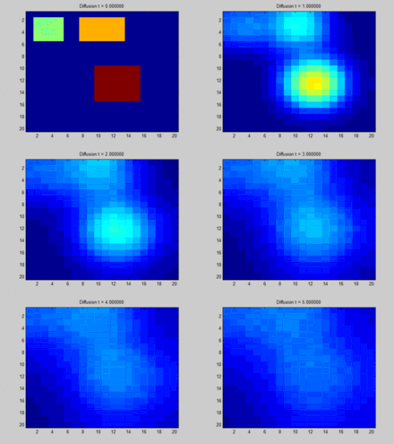
This section shows an example of a function $\phi$ diffusing over time through a graph. The graph in this example is constructed on a 2D discrete grid, with points on the grid connected to their eight neighbors. Three initial points are specified to have a positive value, while the rest of the values in the grid are zero. Over time, the exponential decay acts to distribute the values at these points evenly throughout the entire grid.

The complete Matlab source code that was used to generate this animation is provided below. It shows the process of specifying initial conditions, projecting these initial conditions onto the eigenvalues of the Laplacian Matrix, and simulating the exponential decay of these projected initial conditions.

N = 20;%The number of pixels along a dimension of the image
A = zeros(N, N);%The image
Adj = zeros(N*N, N*N);%The adjacency matrix
 
%Use 8 neighbors, and fill in the adjacency matrix
dx = [-1, 0, 1, -1, 1, -1, 0, 1];
dy = [-1, -1, -1, 0, 0, 1, 1, 1];
for x = 1:N
   for y = 1:N
       index = (x-1)*N + y;
       for ne = 1:length(dx)
           newx = x + dx(ne);
           newy = y + dy(ne);
           if newx > 0 && newx <= N && newy > 0 && newy <= N
               index2 = (newx-1)*N + newy;
               Adj(index, index2) = 1;
           end
       end
   end
end
 
%%%BELOW IS THE KEY CODE THAT COMPUTES THE SOLUTION TO THE DIFFERENTIAL
%%%EQUATION
Deg = diag(sum(Adj, 2));%Compute the degree matrix
L = Deg - Adj;%Compute the laplacian matrix in terms of the degree and adjacency matrices
[V, D] = eig(L);%Compute the eigenvalues/vectors of the laplacian matrix
D = diag(D);
 
%Initial condition (place a few large positive values around and
%make everything else zero)
C0 = zeros(N, N);
C0(2:5, 2:5) = 5;
C0(10:15, 10:15) = 10;
C0(2:5, 8:13) = 7;
C0 = C0(:);
 
C0V = V'*C0;%Transform the initial condition into the coordinate system 
%of the eigenvectors
for t = 0:0.05:5
   %Loop through times and decay each initial component
   Phi = C0V.*exp(-D*t);%Exponential decay for each component
   Phi = V*Phi;%Transform from eigenvector coordinate system to original coordinate system
   Phi = reshape(Phi, N, N);
   %Display the results and write to GIF file
   imagesc(Phi);
   caxis([0, 10]);
   title(sprintf('Diffusion t = %3f', t));
   frame = getframe(1);
   im = frame2im(frame);
   [imind, cm] = rgb2ind(im, 256);
   if t == 0
      imwrite(imind, cm, 'out.gif', 'gif', 'Loopcount', inf, 'DelayTime', 0.1); 
   else
      imwrite(imind, cm, 'out.gif', 'gif', 'WriteMode', 'append', 'DelayTime', 0.1);
   end
end

Approximation to the negative continuous Laplacian

The graph Laplacian matrix can be further viewed as a matrix form of an approximation to the (positive semi-definite) Laplacian operator obtained by the finite difference method.^[6] In this interpretation, every graph vertex is treated as a grid point; the local connectivity of the vertex determines the finite difference approximation stencil at this grid point, the grid size is always one for every edge, and there are no constraints on any grid points, which corresponds to the case of the homogeneous Neumann boundary condition, i.e., free boundary.

References

↑ 1.0 1.1 Weisstein, Eric W., "Laplacian Matrix", MathWorld.
↑ "The Deformed Consensus Protocol", F. Morbidi, Automatica, vol. 49, n. 10, pp. 3049-3055, October 2013.
↑ Chung, Fan R.K. (1997). Spectral graph theory (Repr. with corr., 2. [pr.] ed.). Providence, RI: American Math. Soc. ISBN 0-8218-0315-8.
↑ Chung, Fan (1997) [1992]. Spectral Graph Theory. American Mathematical Society. ISBN 0821803158.
↑ Newman, Mark (2010). Networks: An Introduction. Oxford University Press. ISBN 0199206651.
↑ Smola, Alexander J.; Kondor, Risi (2003), "Kernels and regularization on graphs", Learning Theory and Kernel Machines: 16th Annual Conference on Learning Theory and 7th Kernel Workshop, COLT/Kernel 2003, Washington, DC, USA, August 24-27, 2003, Proceedings, Lecture Notes in Computer Science 2777, Springer, pp. 144–158, doi:10.1007/978-3-540-45167-9_12 .

T. Sunada, Discrete geometric analysis, Proceedings of Symposia in Pure Mathematics, (ed. by P. Exner, J. P. Keating, P. Kuchment, T. Sunada, A. Teplyaev), 77 (2008), 51-86.
B. Bollobaás, Modern Graph Theory, Springer-Verlag (1998, corrected ed. 2013), ISBN 0-387-98488-7, Chapters II.3 (Vector Spaces and Matrices Associated with Graphs), VIII.2 (The Adjacency Matrix and the Laplacian), IX.2 (Electrical Networks and Random Walks).