Laplace distribution
|
Probability density function
| |
|
Cumulative distribution function
| |
| Parameters |
 location (real) location (real) scale (real) scale (real) |
|---|---|
| Support |
 |
 | |
| CDF |
![\begin{cases}
\frac12 \exp \left( \frac{x-\mu}{b} \right) & \mbox{if }x < \mu
\\[8pt]
1-\frac12 \exp \left( -\frac{x-\mu}{b} \right) & \mbox{if }x \geq \mu
\end{cases}](../I/m/e823bb03bef12781b0db110ec123c63c.png) |
| Mean |
|
| Median |
|
| Mode |
|
| Variance |
 |
| Skewness |
 |
| Ex. kurtosis |
 |
| Entropy |
 |
| MGF |
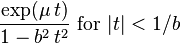 |
| CF |
 |

In probability theory and statistics, the Laplace distribution is a continuous probability distribution named after Pierre-Simon Laplace. It is also sometimes called the double exponential distribution, because it can be thought of as two exponential distributions (with an additional location parameter) spliced together back-to-back, although the term 'double exponential distribution' is also sometimes used to refer to the Gumbel distribution. The difference between two independent identically distributed exponential random variables is governed by a Laplace distribution, as is a Brownian motion evaluated at an exponentially distributed random time. Increments of Laplace motion or a variance gamma process evaluated over the time scale also have a Laplace distribution.
Characterization
Probability density function
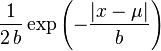
A random variable has a Laplace(μ, b) distribution if its probability density function is
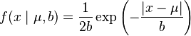
![= \frac{1}{2b}
\left\{\begin{matrix}
\exp \left( -\frac{\mu-x}{b} \right) & \text{if }x < \mu
\\[8pt]
\exp \left( -\frac{x-\mu}{b} \right) & \text{if }x \geq \mu
\end{matrix}\right.](../I/m/51456932550b6013325229dc859735ed.png)
Here, μ is a location parameter and b > 0, which is sometimes referred to as the diversity, is a scale parameter. If μ = 0 and b = 1, the positive half-line is exactly an exponential distribution scaled by 1/2.
The probability density function of the Laplace distribution is also reminiscent of the normal distribution; however, whereas the normal distribution is expressed in terms of the squared difference from the mean μ, the Laplace density is expressed in terms of the absolute difference from the mean. Consequently the Laplace distribution has fatter tails than the normal distribution.
Differential equation
The pdf of the Laplace distribution is a solution of the following differential equation:
![\begin{cases}
\left\{\begin{array}{l}
b f'(x)+f(x)=0 \\[8pt]
f(0)=\frac{e^{\frac{\mu}{b}}}{2b}\end{array}\right\} & \text{if } x \geq \mu \\[8pt]
\left\{\begin{array}{l}
b f'(x)-f(x)=0 \\[8pt]
f(0)=\frac{e^{-\frac{\mu}{b}}}{2b}\end{array}\right\} & \text{if } x < \mu
\end{cases}](../I/m/b81fdd429afe338bd562c24187f686b8.png)
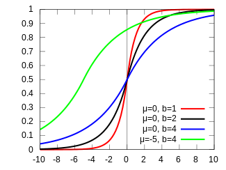
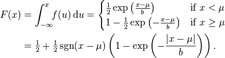
Cumulative distribution function
The Laplace distribution is easy to integrate (if one distinguishes two symmetric cases) due to the use of the absolute value function. Its cumulative distribution function is as follows:
The inverse cumulative distribution function is given by

Generating random variables according to the Laplace distribution
Given a random variable U drawn from the uniform distribution in the interval (−1/2, 1/2], the random variable

has a Laplace distribution with parameters μ and b. This follows from the inverse cumulative distribution function given above.
A Laplace(0, b) variate can also be generated as the difference of two i.i.d. Exponential(1/b) random variables. Equivalently, a Laplace(0, 1) random variable can be generated as the logarithm of the ratio of two iid uniform random variables.
Parameter estimation
Given N independent and identically distributed samples x1, x2, ..., xN, the maximum likelihood estimator  of μ is the sample median,[1]
and the maximum likelihood estimator of b is
of μ is the sample median,[1]
and the maximum likelihood estimator of b is
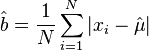
(revealing a link between the Laplace distribution and least absolute deviations).
Moments
![\mu_r' = \bigg({\frac{1}{2}}\bigg) \sum_{k=0}^r \bigg[{\frac{r!}{k! (r-k)!}} b^k \mu^{(r-k)} k! \{1 + (-1)^k\}\bigg]](../I/m/79014853bc474b0a516b0fad86c456df.png)
Related distributions
- If X ~ Laplace(μ, b) then kX + c ~ Laplace(kμ + c, kb).
- If X ~ Laplace(0, b) then |X| ~ Exponential(b−1).
- If X, Y ~ Exponential(λ) then X − Y ~ Laplace(0, λ−1) .
- If X ~ Laplace(μ, b) then |X − μ| ~ Exponential(b−1).
- If X ~ Laplace(μ, b) then X ~ EPD(μ, b, 0).
- If X1, ... X4 ~ N(0, 1) then X1X2 − X3X4 ~ Laplace(0, 1).
- If Xi ~ Laplace(μ, b) then
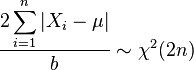 (Chi-squared distribution)
 - If X, Y ~ Laplace(μ, b) then
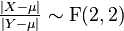 (F-distribution)
 - If X, Y ~ U(0, 1) then log(X/Y) ~ Laplace(0, 1).
- If X ~ Exponential(λ) and Y ~ Bernoulli(0.5) independent of X, then X(2Y − 1) ~ Laplace(0, λ−1).
- If X ~ Exponential(λ) and Y ~ Exponential(ν) independent of X, then λX − νY ~ Laplace(0, 1) .
- If X has a Rademacher distribution and Y ~ Exp(λ) then XY ~ Laplace(0, 1/λ)
- If V ~ Exponential(1) and Z ~ N(0, 1) independent of V, then
 .
. - If X ~ GeometricStable(2, 0, λ, 0) then X ~ Laplace(0, λ).
- The Laplace distribution is a limiting case of the hyperbolic distribution.
- If X|Y ~ Normal(μ, σ = Y) with Y ~ Rayleigh(b) then X ~ Laplace(μ, b).
Relation to the exponential distribution
A Laplace random variable can be represented as the difference of two iid exponential random variables.[2] One way to show this is by using the characteristic function approach. For any set of independent continuous random variables, for any linear combination of those variables, its characteristic function (which uniquely determines the distribution) can be acquired by multiplying the corresponding characteristic functions.
Consider two i.i.d random variables X, Y ~ Exponential(λ). The characteristic functions for X, −Y are
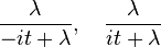
respectively. On multiplying these characteristic functions (equivalent to the characteristic function of the sum of therandom variables X + (−Y)), the result is
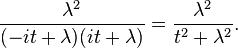
This is the same as the characteristic function for Z ~ Laplace(0,1/λ), which is

Sargan distributions
Sargan distributions are a system of distributions of which the Laplace distribution is a core member. A pth order Sargan distribution has density[3][4]
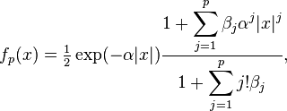
for parameters α ≥ 0, βj ≥ 0. The Laplace distribution results for p = 0.
Applications
The Laplacian distribution has been used in speech recognition to model priors on DFT coefficients.[5]
The addition of noise drawn from a Laplacian distribution, with scaling parameter appropriate to a function's sensitivity, to the output of a statistical database query is the most common means to provide differential privacy in statistical databases.
The least absolute deviations estimate arises as the maximum likelihood estimate if the errors have a Laplace distribution.
History
This distribution is often referred to as Laplace's first law of errors. He published it in 1774 when he noted that the frequency of an error could be expressed as an exponential function of its magnitude once its sign was disregarded.[6][7]
Keynes published a paper in 1911 based on his earlier thesis wherein he showed that the Laplace distribution minimised the absolute deviation from the median.[8]
See also
- Log-Laplace distribution
- Cauchy distribution, also called the "Lorentzian distribution" (the Fourier transform of the Laplace)
- Characteristic function (probability theory)
References
- ↑ Robert M. Norton (May 1984). "The Double Exponential Distribution: Using Calculus to Find a Maximum Likelihood Estimator". The American Statistician (American Statistical Association) 38 (2): 135–136. doi:10.2307/2683252. JSTOR 2683252.
- ↑ Kotz, Samuel; Kozubowski, Tomasz J.; Podgórski, Krzysztof (2001). The Laplace distribution and generalizations: a revisit with applications to Communications, Economics, Engineering and Finance. Birkhauser. pp. 23 (Proposition 2.2.2, Equation 2.2.8). ISBN 9780817641665.
- ↑ Everitt, B.S. (2002) The Cambridge Dictionary of Statistics, CUP. ISBN 0-521-81099-X
- ↑ Johnson, N.L., Kotz S., Balakrishnan, N. (1994) Continuous Univariate Distributions, Wiley. ISBN 0-471-58495-9. p. 60
- ↑ Eltoft, T.; Taesu Kim; Te-Won Lee (2006). "On the multivariate Laplace distribution". IEEE Signal Processing Letters 13 (5): 300–303. doi:10.1109/LSP.2006.870353.
- ↑ Laplace, P-S. (1774). Mémoire sur la probabilité des causes par les évènements. Mémoires de l’Academie Royale des Sciences Presentés par Divers Savan, 6, 621–656
- ↑ Wilson EB (1923) First and second laws of error. JASA 18, 143
- ↑ Keynes JM (1911) The principal averages and the laws of error which lead to them. J Roy Stat Soc, 74, 322–331
External links
- Hazewinkel, Michiel, ed. (2001), "Laplace distribution", Encyclopedia of Mathematics, Springer, ISBN 978-1-55608-010-4
| ||||||||||||||