LCP array
| LCP array | ||
|---|---|---|
| Type | Array | |
| Invented by | Manber & Myers (1990) | |
| Time complexity and space complexity in big O notation | ||
| Average | Worst case | |
| Space |  |
|
| Construction | |
|
In computer science, the longest common prefix array (LCP array) is an auxiliary data structure to the suffix array. It stores the lengths of the longest common prefixes between pairs of consecutive suffixes in the sorted suffix array. In other words, it is the length of prefix that is common between the two consecutive suffixes in a sorted suffix array.
Example:
LCP of a and aabba is 1.
LCP of abaabba and abba is 2.
Augmenting the suffix array with the LCP array allows to efficiently simulate top-down and bottom-up traversals of the suffix tree,[1][2] speeds up pattern matching on the suffix array[3] and is a prerequisite for compressed suffix trees.[4]
History
The LCP array was introduced by Udi Manber and Gene Myers alongside the suffix array in order to improve the running time of their string search algorithm.[3]
Gene Myers was the former Vice president of Informatics Research at Celera Genomics, and Udi Manber was vice president of engineering at Google.
Definition
Let  be the suffix array of the string
  and let
  denote the length of the longest common prefix between two strings
  and
and  . Let further denote
 ![S[i,j]](../I/m/da0ee77c5e0b0b1163aeae0fb43fbaad.png) the substring of
the substring of  ranging from
  to
to  .
.
Then the LCP array ![H[1,n]](../I/m/a67b1c16fea0e75d333f0725add3bdb6.png) is an integer array of size
is an integer array of size  such that
 ![H[1]](../I/m/9ee660f8c5ac88dc78a6200d677a6b43.png) is undefined and
is undefined and ![H[i]=\operatorname{lcp}(S[A[i-1],n],S[A[i],n])](../I/m/a27383d14d2aef1893f3335549b2868d.png) for every
for every  . Thus
 ![H[i]](../I/m/08f9c9d30750bf03ac5ff958956449c6.png) stores the length of longest common prefix of the lexicographically 'th smallest suffix and its predecessor in the suffix array.
stores the length of longest common prefix of the lexicographically 'th smallest suffix and its predecessor in the suffix array.
Example
Consider the string  :
:
| i | 1 | 2 | 3 | 4 | 5 | 6 | 7 |
|---|---|---|---|---|---|---|---|
| S[i] | b | a | n | a | n | a | $ |
and its corresponding suffix array :
| i | 1 | 2 | 3 | 4 | 5 | 6 | 7 |
|---|---|---|---|---|---|---|---|
| A[i] | 7 | 6 | 4 | 2 | 1 | 5 | 3 |
Complete suffix array with suffixes itself :
| i | 1 | 2 | 3 | 4 | 5 | 6 | 7 |
|---|---|---|---|---|---|---|---|
| A[i] | 7 | 6 | 4 | 2 | 1 | 5 | 3 |
| 1 | $ | a | a | a | b | n | n |
| 2 | $ | n | n | a | a | a | |
| 3 | a | a | n | $ | n | ||
| 4 | $ | n | a | a | |||
| 5 | a | n | $ | ||||
| 6 | $ | a | |||||
| 7 | $ |
Then the LCP array  is constructed by comparing lexicographically consecutive suffixes to determine their longest common prefix:
| i | 1 | 2 | 3 | 4 | 5 | 6 | 7 |
|---|---|---|---|---|---|---|---|
| H[i] |  | 0 | 1 | 3 | 0 | 0 | 2 |
So, for example, ![H[4]=3](../I/m/4c3b25f55e8c698ab6028ab871b9b264.png) is the length of the longest common prefix
is the length of the longest common prefix  shared by the suffixes
 ![A[3]=S[4,7]=ana$](../I/m/e3f63237447d1047a0963242288b95a0.png) and
and ![A[4]=S[2,7]=anana$](../I/m/31fc78cf263a4cdc887e9200d736883b.png) . Note that
. Note that ![H[1]=\bot](../I/m/0a3565b0e1a804935c7604a4e1ca84dc.png) , since there is no lexicographically smaller suffix.
, since there is no lexicographically smaller suffix.
Difference between Suffix Array and LCP Array?
Suffix array: Represents the lexicographic rank of each suffix of an array.
LCP array: Contains the maximum length prefix match between two consecutive suffixes, after they are sorted lexicographically.
LCP Array usage in finding the number of occurrences of a pattern
In order to find the number of occurrences of a given string P (length m) in a text T (length N),
- You must use binary search against the suffix array of T.
- You should speed up the LCP array usage as an auxiliary data structure. More specifically, you generate a special version of the LCP array (LCP-LR below) and use that.
The issue with using standard binary search (without the LCP information) is that in each of the O(log N) comparisons you need to make, you compare P to the current entry of the suffix array, which means a full string comparison of up to m characters. So the complexity is O(m*log N).
The LCP-LR array helps improve this to O(m+log N), in the following way:
At any point during the binary search algorithm, you consider, as usual, a range (L,...,R) of the suffix array and its central point M, and decide whether you continue your search in the left sub-range (L,...,M) or in the right sub-range (M,...,R). In order to make the decision, you compare P to the string at M. If P is identical to M, you are done, but if not, you will have compared the first k characters of P and then decided whether P is lexicographically smaller or larger than M. Let's assume the outcome is that P is larger than M. So, in the next step, you consider (M,...,R) and a new central point M' in the middle:
             M ...... M' ...... R
             |
      we know:
         lcp(P,M)==k
The trick now is that LCP-LR is precomputed such that an O(1)-lookup tells you the longest common prefix of M and M', lcp(M,M').
You know already (from the previous step) that M itself has a prefix of k characters in common with P: lcp(P,M)=k. Now there are three possibilities:
- Case 1: k < lcp(M,M'), i.e. P has fewer prefix characters in common with M than M has in common with M'. This means the (k+1)-th character of M' is the same as that of M, and since P is lexicographically larger than M, it must be lexicographically larger than M', too. So we continue in the right half (M',...,R).
- Case 2: k > lcp(M,M'), i.e. P has more prefix characters in common with M than M has in common with M'. Consequently, if we were to compare P to M', the common prefix would be smaller than k, and M' would be lexicographically larger than P, so, without actually making the comparison, we continue in the left half (M,...,M').
- Case 3: k == lcp(M,M'). So M and M' are both identical with P in the first k characters. To decide whether we continue in the left or right half, it suffices to compare P to M' starting from the (k+1)-th character.
- We continue recursively.
The overall effect is that no character of P is compared to any character of the text more than once. The total number of character comparisons is bounded by m, so the total complexity is indeed O(m+log N).
Obviously, the key remaining question is how did we precompute LCP-LR so it is able to tell us in O(1) time the lcp between any two entries of the suffix array? As you said, the standard LCP array tells you the lcp of consecutive entries only, i.e. lcp(x-1,x) for any x. But M and M' in the description above are not necessarily consecutive entries, so how is that done?
The key to this is to realize that only certain ranges (L,...,R) will ever occur during the binary search: It always starts with (0,...,N) and divides that at the center, and then continues either left or right and divide that half again and so forth. If you think of it: Every entry of the suffix array occurs as central point of exactly one possible range during binary search. So there are exactly N distinct ranges (L...M...R) that can possibly play a role during binary search, and it suffices to precompute lcp(L,M) and lcp(M,R) for those N possible ranges. So that is 2*N distinct precomputed values, hence LCP-LR is O(N) in size.
Moreover, there is a straightforward recursive algorithm to compute the 2*N values of LCP-LR in O(N) time from the standard LCP array – I'd suggest posting a separate question if you need a detailed description of that.
To sum up:
- It is possible to compute LCP-LR in O(N) time and O(2*N)=O(N) space from LCP.
- Using LCP-LR during binary search helps accelerate the search procedure from O(M*log N) to O(M+log N).
- You can use two binary searches to determine the left and right end of the match range for P, and the length of the match range corresponds with the number of occurrences for P.
Efficient Construction Algorithms
LCP array construction algorithms can be divided into two different categories: algorithms that compute the LCP array as a byproduct to the suffix array and algorithms that use an already constructed suffix array in order to compute the LCP values.
Manber & Myers (1993) provide an algorithm to compute the LCP array alongside the suffix array
in  time. Kärkkäinen & Sanders (2003) show that it is also possible to modify their
 time algorithm such that it computes the LCP array as well.
Kasai et al. (2001) present the first time algorithm (FLAAP) that computes the LCP
array given the text and the suffix array.
time algorithm such that it computes the LCP array as well.
Kasai et al. (2001) present the first time algorithm (FLAAP) that computes the LCP
array given the text and the suffix array.
Assuming that each text symbol takes
one byte and each entry of the suffix or LCP array takes 4 bytes, the major drawback of their
algorithm is a large space occupancy of  bytes, while the
original output (text, suffix array, LCP array) only occupies
bytes, while the
original output (text, suffix array, LCP array) only occupies  bytes. Therefore Manzini (2004) created a refined version of the algorithm of Kasai et al. (2001) (lcp9) and reduced the
space occupancy to bytes. Kärkkäinen, Manzini & Puglisi (2009) provide another refinement of
Kasai's algorithm (
bytes. Therefore Manzini (2004) created a refined version of the algorithm of Kasai et al. (2001) (lcp9) and reduced the
space occupancy to bytes. Kärkkäinen, Manzini & Puglisi (2009) provide another refinement of
Kasai's algorithm ( -algorithm) that improves the running
time. Rather than the actual LCP array, this algorithm builds the permuted
LCP (PLCP) array, in which the values appear in text order rather than lexicographical order.
-algorithm) that improves the running
time. Rather than the actual LCP array, this algorithm builds the permuted
LCP (PLCP) array, in which the values appear in text order rather than lexicographical order.
Gog & Ohlebusch (2011) provide two algorithms that although being theoretically slow
( ) were faster than the above mentioned algorithms in
practice.
) were faster than the above mentioned algorithms in
practice.
As of 2012, the currently fastest linear-time LCP array construction algorithm is due to Fischer (2011), which in turn is based on one of the fastest suffix array construction algorithms by Nong, Zhang & Chan (2009).
Applications
As noted by Abouelhoda, Kurtz & Ohlebusch (2004) several string processing problems can be solved by the following kinds of tree traversals:
- bottom-up traversal of the complete suffix tree
- top-down traversal of a subtree of the suffix tree
- suffix tree traversal using the suffix links.
Kasai et al. (2001) show how to simulate a bottom-up traversal of the suffix tree using only the suffix array and LCP array. Abouelhoda, Kurtz & Ohlebusch (2004) enhance the suffix array with the LCP array and additional data structures and describe how this enhanced suffix array can be used to simulate all three kinds of suffix tree traversals. Fischer & Heun (2007) reduce the space requirements of the enhanced suffix array by preprocessing the LCP array for range minimum queries. Thus, every problem that can be solved by suffix tree algorithms can also be solved using the enhanced suffix array.[2]
Deciding if a pattern  of length
  is a substring of a string of length takes
  time if only the suffix array is used. By additionally using the LCP information, this bound can be improved to
  time.[3] Abouelhoda, Kurtz & Ohlebusch (2004) show how to improve this running time even further to achieve optimal
  time. Thus, using suffix array and LCP array information, the decision query can be answered as fast as using the suffix tree.
The LCP array is also an essential part of compressed suffix trees which provide full suffix tree functionality like suffix links and lowest common ancestor queries.[5][6] Furthermore it can be used together with the suffix array to compute the Lempel-Ziv LZ77 factorization in time. [2][7][8][9]
The longest repeated substring problem for a string of length can be solved in  time using both the suffix array and the LCP array. It is sufficient to perform a linear scan through the LCP array in order to find its maximum value
  and the corresponding index where is stored. The longest substring that occurs at least twice is then given by
 ![S[A[i],A[i]+v_{max}-1]](../I/m/3fbf239c40f0b6060a219e4a35773225.png) .
.
The remainder of this section explains two applications of the LCP array in more detail: How the suffix array and the LCP array of a string can be used to construct the corresponding suffix tree and how it is possible to answer LCP queries for arbitrary suffixes using range minimum queries on the LCP array.
Suffix tree construction
Given the suffix array and the LCP array of a string of length  , its suffix tree
  can be constructed in time based on the following idea: Start with the partial suffix tree for the lexicographically smallest suffix and repeatedly insert the other suffixes in the order given by the suffix array.
Let  be the partial suffix tree for
  . Further let
  be the length of the concatenation of all path labels from the root of
  to node .
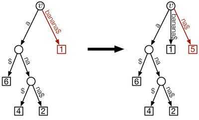
![d(v)=H[i+1]](../I/m/d775a135ed082b62fa31256d195d4f9e.png) ): Suppose the suffixes
): Suppose the suffixes  ,
,  ,
,  and
and  of the string are already added to the suffix tree. Then the suffix
  is added to the tree as shown in the picture. The rightmost path is highlighted in red.
Start with  , the tree consisting only of the root. To insert
 ![A[i+1]](../I/m/7c32aab82d95eb6cfacf9559b3b1f14f.png) into , walk up the rightmost path beginning at the recently inserted leaf
into , walk up the rightmost path beginning at the recently inserted leaf ![A[i]](../I/m/8a6b5ab46e06fa60418f7c34e624b076.png) to the root, until the deepest node with
to the root, until the deepest node with ![d(v) \leq H[i+1]](../I/m/a562c52bc02fd2c59d578fbff0f8af0a.png) is reached.
is reached.
We need to distinguish two cases:
- : This means that the concatenation of the labels on the root-to- path equals the longest common prefix of suffixes and .
In this case, insert as a new leaf  of node and label the edge
  with
with ![S[A[i+1]+H[i+1],n]](../I/m/856e7bc0332b534039b67ddcb0c29e00.png) . Thus the edge label consists of the remaining characters of suffix that are not already represented by the concatenation of the labels of the root-to- path.
. Thus the edge label consists of the remaining characters of suffix that are not already represented by the concatenation of the labels of the root-to- path.
This creates the partial suffix tree .
. 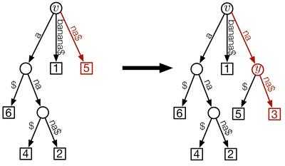 Case 2 (
![d(v) < H[i+1]](../I/m/e2bcedc895fa55603a4543ded3660cc1.png) ): In order to add suffix
): In order to add suffix  , the edge to the previously inserted suffix has to be split up. The new edge to the new internal node is labeled with the longest common prefix of the suffixes and . The edges connecting the two leaves are labeled with the remaining suffix characters that are not part of the prefix.
- : This means that the concatenation of the labels on the root-to- path displays less characters than the longest common prefix of suffixes and and the missing characters are contained in the edge label of 's rightmost edge. Therefore we have to split up that edge as follows:
Let be the child of on 's rightmost path.
- Delete the edge
 .
. - Add a new internal node
 and a new edge
  with label
 ![S[A[i]+d(v),A[i]+H[i+1]-1]](../I/m/489b13f7fb9a299c3d5c385dc08d1af4.png) . The new label consists of the missing characters of the longest common prefix of and . Thus, the concatenation of the labels of the root-to- path now displays the longest common prefix of and .
. The new label consists of the missing characters of the longest common prefix of and . Thus, the concatenation of the labels of the root-to- path now displays the longest common prefix of and . - Connect to the newly created internal node by an edge
 that is labeled
 ![S[A[i]+H[i+1],A[i]+d(w)-1]](../I/m/b19ce4d91cca43dfbd9ea833084b9da2.png) . The new label consists of the remaining characters of the deleted edge that were not used as the label of edge .
. The new label consists of the remaining characters of the deleted edge that were not used as the label of edge . - Add as a new leaf and connect it to the new internal node by an edge
 that is labeled . Thus the edge label consists of the remaining characters of suffix that are not already represented by the concatenation of the labels of the root-to- path.
 - This creates the partial suffix tree .
A simple amortization argument shows that the running time of this algorithm is bounded by :
The nodes that are traversed in step by walking up the rightmost path of (apart from the last node ) are removed from the rightmost path, when is added to the tree as a new leaf. These nodes will never be traversed again for all subsequent steps  . Therefore, at most
  nodes will be traversed in total.
LCP queries for arbitrary suffixes
The LCP array only contains the length of the longest common prefix of every pair of consecutive suffixes in the suffix array . However, with the help of the inverse suffix array  (
(![A[i]= j \Leftrightarrow A^{-1}[j]= i](../I/m/6f2f1fe96822ada0fd35514d8d214adb.png) , i.e. the suffix
, i.e. the suffix ![S[j,n]](../I/m/8e919a854707b0a0ed1f14abc606ff71.png) that starts at position in is stored in position
that starts at position in is stored in position ![A^{-1}[j]](../I/m/5d46353e96d07d1e0774cd120cc1aba5.png) in ) and constant-time range minimum queries on , it is possible to determine the length of the longest common prefix of arbitrary suffixes in
in ) and constant-time range minimum queries on , it is possible to determine the length of the longest common prefix of arbitrary suffixes in  time.
time.
Because of the lexicographic order of the suffix array, every common prefix of the suffixes ![S[i,n]](../I/m/1a16fb018d6deada23b0d6f36f4d4ccf.png) and has to be a common prefix of all suffixes between 's position in the suffix array
and has to be a common prefix of all suffixes between 's position in the suffix array ![A^{-1}[i]](../I/m/9fde9f9b6b90bbd6fa89be485beecccb.png) and 's position in the suffix array . Therefore the length of the longest prefix that is shared by all of these suffixes is the minimum value in the interval
and 's position in the suffix array . Therefore the length of the longest prefix that is shared by all of these suffixes is the minimum value in the interval ![H[A^{-1}[i]+1,A^{-1}[j]]](../I/m/f4a55cbe8dfcf59566c732b42a1e1d75.png) . This value can be found in constant time if is preprocessed for range minimum queries.
. This value can be found in constant time if is preprocessed for range minimum queries.
Thus given a string of length and two arbitrary positions  in the string with
 ![A^{-1}[i] < A^{-1}[j]](../I/m/5d254db78b5c44d0cba01eafc5dc1af9.png) , the length of the longest common prefix of the suffixes and can be computed as follows:
, the length of the longest common prefix of the suffixes and can be computed as follows: ![\operatorname{LCP}(i,j)=H[\operatorname{RMQ}_H(A^{-1}[i]+1,A^{-1}[j])]](../I/m/0c8e0702771775d433ed185bbd49a514.png) .
.
Notes
References
- Abouelhoda, Mohamed Ibrahim; Kurtz, Stefan; Ohlebusch, Enno (2004). "Replacing suffix trees with enhanced suffix arrays". Journal of Discrete Algorithms 2: 53. doi:10.1016/S1570-8667(03)00065-0.
- Manber, Udi; Myers, Gene (1993). "Suffix Arrays: A New Method for On-Line String Searches". SIAM Journal on Computing 22 (5): 935. doi:10.1137/0222058.
- Kasai, T.; Lee, G.; Arimura, H.; Arikawa, S.; Park, K. (2001). Linear-Time Longest-Common-Prefix Computation in Suffix Arrays and Its Applications. Proceedings of the 12th Annual Symposium on Combinatorial Pattern Matching. Lecture Notes in Computer Science 2089. pp. 181–192. doi:10.1007/3-540-48194-X_17. ISBN 978-3-540-42271-6.
- Ohlebusch, Enno; Fischer, Johannes; Gog, Simon (2010). CST++. String Processing and Information Retrieval. Lecture Notes in Computer Science 6393. p. 322. doi:10.1007/978-3-642-16321-0_34. ISBN 978-3-642-16320-3.
- Kärkkäinen, Juha; Sanders, Peter (2003). Simple linear work suffix array construction. Proceedings of the 30th international conference on Automata, languages and programming. pp. 943–955. Retrieved 2012-08-28.
- Fischer, Johannes (2011). Inducing the LCP-Array. Algorithms and Data Structures. Lecture Notes in Computer Science 6844. pp. 374–385. doi:10.1007/978-3-642-22300-6_32. ISBN 978-3-642-22299-3.
- Manzini, Giovanni (2004). Two Space Saving Tricks for Linear Time LCP Array Computation. Algorithm Theory - SWAT 2004. Lecture Notes in Computer Science 3111. p. 372. doi:10.1007/978-3-540-27810-8_32. ISBN 978-3-540-22339-9.
- Kärkkäinen, Juha; Manzini, Giovanni; Puglisi, Simon J. (2009). Permuted Longest-Common-Prefix Array. Combinatorial Pattern Matching. Lecture Notes in Computer Science 5577. p. 181. doi:10.1007/978-3-642-02441-2_17. ISBN 978-3-642-02440-5.
- Puglisi, Simon J.; Turpin, Andrew (2008). Space-Time Tradeoffs for Longest-Common-Prefix Array Computation. Algorithms and Computation. Lecture Notes in Computer Science 5369. p. 124. doi:10.1007/978-3-540-92182-0_14. ISBN 978-3-540-92181-3.
- Gog, Simon; Ohlebusch, Enno (2011). Fast and Lightweight LCP-Array Construction Algorithms (PDF). Proceedings of the Workshop on Algorithm Engineering and Experiments, ALENEX 2011. pp. 25–34. Retrieved 2012-08-28.
- Nong, Ge; Zhang, Sen; Chan, Wai Hong (2009). Linear Suffix Array Construction by Almost Pure Induced-Sorting. 2009 Data Compression Conference. p. 193. doi:10.1109/DCC.2009.42. ISBN 978-0-7695-3592-0.
- Fischer, Johannes; Heun, Volker (2007). A New Succinct Representation of RMQ-Information and Improvements in the Enhanced Suffix Array. Combinatorics, Algorithms, Probabilistic and Experimental Methodologies. Lecture Notes in Computer Science 4614. p. 459. doi:10.1007/978-3-540-74450-4_41. ISBN 978-3-540-74449-8.
- Chen, G.; Puglisi, S. J.; Smyth, W. F. (2008). "Lempel–Ziv Factorization Using Less Time & Space". Mathematics in Computer Science 1 (4): 605. doi:10.1007/s11786-007-0024-4.
- Crochemore, M.; Ilie, L. (2008). "Computing Longest Previous Factor in linear time and applications". Information Processing Letters 106 (2): 75. doi:10.1016/j.ipl.2007.10.006.
- Crochemore, M.; Ilie, L.; Smyth, W. F. (2008). A Simple Algorithm for Computing the Lempel Ziv Factorization. Data Compression Conference (dcc 2008). p. 482. doi:10.1109/DCC.2008.36. ISBN 978-0-7695-3121-2.
- Sadakane, K. (2007). "Compressed Suffix Trees with Full Functionality". Theory of Computing Systems 41 (4): 589–607. doi:10.1007/s00224-006-1198-x.
External links
- Mirror of the ad-hoc-implementation of the code described in Fischer (2011)
- SDSL: Succinct Data Structure Library - Provides various LCP array implementations, Range Minimum Query (RMQ) support structures and many more succinct data structures
- Bottom-up suffix tree traversal emulated using suffix array and LCP array (Java)
- Text-Indexing project (linear-time construction of suffix trees, suffix arrays, LCP array and Burrows-Wheeler Transform)