Kirchhoff–Love plate theory

The Kirchhoff–Love theory of plates is a two-dimensional mathematical model that is used to determine the stresses and deformations in thin plates subjected to forces and moments. This theory is an extension of Euler-Bernoulli beam theory and was developed in 1888 by Love[1] using assumptions proposed by Kirchhoff. The theory assumes that a mid-surface plane can be used to represent a three-dimensional plate in two-dimensional form.
The following kinematic assumptions that are made in this theory:[2]
- straight lines normal to the mid-surface remain straight after deformation
- straight lines normal to the mid-surface remain normal to the mid-surface after deformation
- the thickness of the plate does not change during a deformation.
Assumed displacement field
Let the position vector of a point in the undeformed plate be  . Then

The vectors  form a Cartesian basis with origin on the mid-surface of the plate,
  and
and  are the Cartesian coordinates on the mid-surface of the undeformed plate, and
  is the coordinate for the thickness direction.
Let the displacement of a point in the plate be  . Then

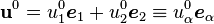
This displacement can be decomposed into a vector sum of the mid-surface displacement and an out-of-plane displacement  in the direction. We can write the in-plane displacement of the mid-surface as
Note that the index  takes the values 1 and 2 but not 3.
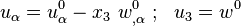
Then the Kirchhoff hypothesis implies that
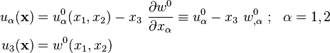
If  are the angles of rotation of the normal to the mid-surface, then in the Kirchhoff-Love theory

Note that we can think of the expression for  as the first order Taylor series expansion of the displacement around the mid-surface.
 Displacement of the mid-surface (left) and of a normal (right) |
Quasistatic Kirchhoff-Love plates
The original theory developed by Love was valid for infinitesimal strains and rotations. The theory was extended by von Kármán to situations where moderate rotations could be expected.
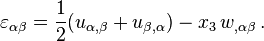
Strain-displacement relations
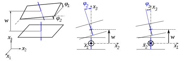
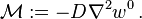
For the situation where the strains in the plate are infinitesimal and the rotations of the mid-surface normals are less than 10° the strain-displacement relations are
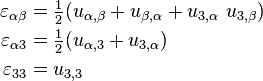
Using the kinematic assumptions we have
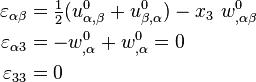
Therefore the only non-zero strains are in the in-plane directions.
Equilibrium equations
The equilibrium equations for the plate can be derived from the principle of virtual work. For a thin plate under a quasistatic transverse load  these equations are
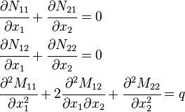
where the thickness of the plate is  . In index notation,
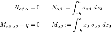
where  are the stresses.
 Bending moments and normal stresses |
 Torques and shear stresses |
Derivation of equilibrium equations for small rotations For the situation where the strains and rotations of the plate are small the virtual internal energy is given by where the thickness of the plate is
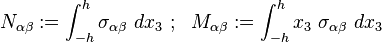
and the stress resultants and stress moment resultants are defined asIntegration by parts leads to
The symmetry of the stress tensor implies that
 . Hence,
Another integration by parts gives
For the case where there are no prescribed external forces, the principle of virtual work implies that
 . The equilibrium equations for the plate are then given by
If the plate is loaded by an external distributed load
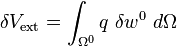
that is normal to the mid-surface and directed in the positive direction, the external virtual work due to the load isThe principle of virtual work then leads to the equilibrium equations
![\begin{align}
\delta U & = \int_{\Omega^0} \int_{-h}^h \boldsymbol{\sigma}:\delta\boldsymbol{\epsilon}~dx_3~d\Omega
= \int_{\Omega^0} \int_{-h}^h \sigma_{\alpha\beta}~\delta\varepsilon_{\alpha\beta}~dx_3~d\Omega \\
& = \int_{\Omega^0} \int_{-h}^h \left[\frac{1}{2}~\sigma_{\alpha\beta}~(\delta u^0_{\alpha,\beta}+\delta u^0_{\beta,\alpha}) - x_3~\sigma_{\alpha\beta}~\delta w^0_{,\alpha\beta}\right]~dx_3~d\Omega \\
& = \int_{\Omega^0} \left[\frac{1}{2}~N_{\alpha\beta}~(\delta u^0_{\alpha,\beta}+\delta u^0_{\beta,\alpha}) - M_{\alpha\beta}~\delta w^0_{,\alpha\beta}\right]~d\Omega
\end{align}](../I/m/d2fc5aa2af4b7345191c6e3785f540d2.png)
![\begin{align}
\delta U & = \int_{\Omega^0} \left[-\frac{1}{2}~(N_{\alpha\beta,\beta}~\delta u^0_{\alpha}+N_{\alpha\beta,\alpha}~\delta u^0_{\beta})
+ M_{\alpha\beta,\beta}~\delta w^0_{,\alpha}\right]~d\Omega \\
& + \int_{\Gamma^0} \left[\frac{1}{2}~(n_\beta~N_{\alpha\beta}~\delta u^0_\alpha+n_\alpha~N_{\alpha\beta}~\delta u^0_{\beta})
- n_\beta~M_{\alpha\beta}~\delta w^0_{,\alpha}\right]~d\Gamma
\end{align}](../I/m/14a8cc930c0cf76ec659b6c574c9e934.png)
![\delta U = \int_{\Omega^0} \left[-N_{\alpha\beta,\alpha}~\delta u^0_{\beta}
+ M_{\alpha\beta,\beta}~\delta w^0_{,\alpha}\right]~d\Omega
+ \int_{\Gamma^0} \left[n_\alpha~N_{\alpha\beta}~\delta u^0_{\beta}
- n_\beta~M_{\alpha\beta}~\delta w^0_{,\alpha}\right]~d\Gamma](../I/m/92acdcf84e988c981c2e920c8d50c6b4.png)
![\delta U = \int_{\Omega^0} \left[-N_{\alpha\beta,\alpha}~\delta u^0_{\beta}
- M_{\alpha\beta,\beta\alpha}~\delta w^0\right]~d\Omega
+ \int_{\Gamma^0} \left[n_\alpha~N_{\alpha\beta}~\delta u^0_{\beta}
+ n_\alpha~M_{\alpha\beta,\beta}~\delta w^0
- n_\beta~M_{\alpha\beta}~\delta w^0_{,\alpha}\right]~d\Gamma](../I/m/af55b69be18e0ad42244dfe2be90c6e9.png)

Boundary conditions
The boundary conditions that are needed to solve the equilibrium equations of plate theory can be obtained from the boundary terms in the principle of virtual work. In the absence of external forces on the boundary, the boundary conditions are
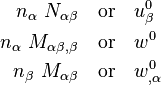
Note that the quantity  is an effective shear force.
Constitutive relations
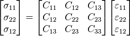
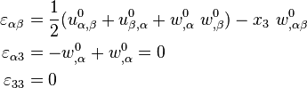
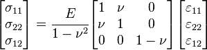
The stress-strain relations for a linear elastic Kirchhoff plate are given by
Since  and
and  do not appear in the equilibrium equations it is implicitly assumed that these quantities do not have any effect on the momentum balance and are neglected. The remaining stress-strain relations, in matrix form, can be written as
Then,

and

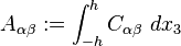
The extensional stiffnesses are the quantities
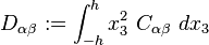
The bending stiffnesses (also called flexural rigidity) are the quantities
The Kirchhoff-Love constitutive assumptions lead to zero shear forces. As a result, the equilibrium equations for the plate have to be used to determine the shear forces in thin Kirchhoff-Love plates. For isotropic plates, these equations lead to
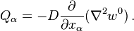
Alternatively, these shear forces can be expressed as

where
Small strains and moderate rotations
If the rotations of the normals to the mid-surface are in the range of 10 to 15
to 15 , the strain-displacement relations can be approximated as
Then the kinematic assumptions of Kirchhoff-Love theory lead to the classical plate theory with von Kármán strains
This theory is nonlinear because of the quadratic terms in the strain-displacement relations.
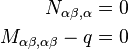
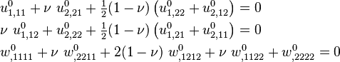
If the strain-displacement relations take the von Karman form, the equilibrium equations can be expressed as
![\begin{align}
N_{\alpha\beta,\alpha} & = 0 \\
M_{\alpha\beta,\alpha\beta} + [N_{\alpha\beta}~w^0_{,\beta}]_{,\alpha} - q & = 0
\end{align}](../I/m/b0540d0fff760e65355373cbb0cf25f8.png)
Isotropic quasistatic Kirchhoff-Love plates
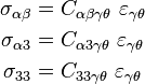
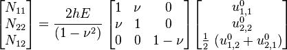
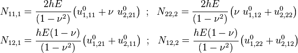
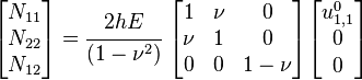
For an isotropic and homogeneous plate, the stress-strain relations are
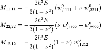
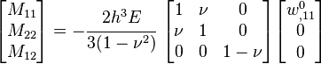
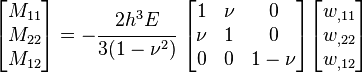
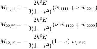
The moments corresponding to these stresses are
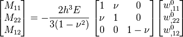
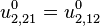
In expanded form,
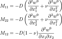
where ![D = 2h^3E/[3(1-\nu^2)] = H^3E/[12(1-\nu^2)]](../I/m/f7a12a170c5ccdbf55ca47f16ae1963e.png) for plates of thickness
for plates of thickness  . Using the stress-strain relations for the plates, we can show that the stresses and moments are related by

At the top of the plate where 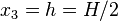 , the stresses are

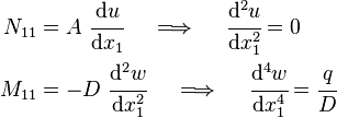
Pure bending
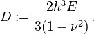
For an isotropic and homogeneous plate under pure bending, the governing equations reduce to
Here we have assumed that the in-plane displacements do not vary with and . In index notation,
and in direct notation

The bending moments are given by
Derivation of equilibrium equations for pure bending For an isotropic, homogeneous plate under pure bending the governing equations are and the stress-strain relations are
Then,
and
Differentiation gives
and
Plugging into the governing equations leads to
Since the order of differentiation is irrelevant we have
 ,
,  , and
, and 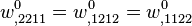 . Hence
In direct tensor notation, the governing equation of the plate is
where we have assumed that the displacements
 are constant.
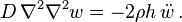
Bending under transverse load
If a distributed transverse load  is applied to the plate, the governing equation is
 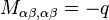 . Following the procedure shown in the previous section we get[3]
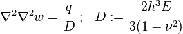
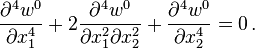
In rectangular Cartesian coordinates, the governing equation is
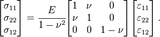
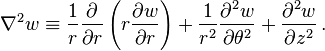
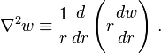
and in cylindrical coordinates it takes the form
![\frac{1}{r}\cfrac{d }{d r}\left[r \cfrac{d }{d r}\left\{\frac{1}{r}\cfrac{d }{d r}\left(r \cfrac{d w}{d r}\right)\right\}\right] = - \frac{q}{D}\,.](../I/m/06fb2af0b5690fed73d532b7e5d10e27.png)
Solutions of this equation for various geometries and boundary conditions can be found in the article on bending of plates.
Derivation of equilibrium equations for transverse loading For a transversely loaded plate without axial deformations, the governing equation has the form where
 is a distributed transverse load (per unit area). Substitution of the expressions for the derivatives of
  into the governing equation gives
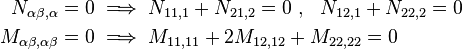
Noting that the bending stiffness is the quantity
we can write the governing equation in the form
In cylindrical coordinates
 ,
,For symmetrically loaded circular plates,
 , and we have
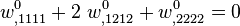
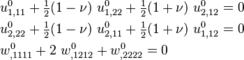

![-\cfrac{2h^3E}{3(1-\nu^2)}\left[w^0_{,1111} + 2\,w^0_{,1212} + w^0_{,2222}\right] = q \,.](../I/m/6d77fe3846b0792964129ab25ddfba7e.png)
Cylindrical bending
Under certain loading conditions a flat plate can be bent into the shape of the surface of a cylinder. This type of bending is called cylindrical bending and represents the special situation where  . In that case
and
and the governing equations become[3]
Dynamics of Kirchhoff-Love plates
The dynamic theory of thin plates determines the propagation of waves in the plates, and the study of standing waves and vibration modes.
Governing equations
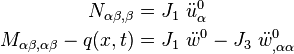
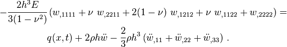
The governing equations for the dynamics of a Kirchhoff-Love plate are
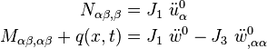
where, for a plate with density  ,
,

and
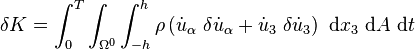
Derivation of equations governing the dynamics of Kirchhoff-Love plates The total kinetic energy of the plate is given by
Therefore the variation in kinetic energy is
We use the following notation in the rest of this section.
Then
For a Kirchhof-Love plate
Hence,
Define, for constant
 through the thickness of the plate,
 Then
Integrating by parts,
The variations
 and
and  are zero at
  and
and  .
Hence, after switching the sequence of integration, we have
.
Hence, after switching the sequence of integration, we haveIntegration by parts over the mid-surface gives
Again, since the variations are zero at the beginning and the end of the time interval under consideration, we have
For the dynamic case, the variation in the internal energy is given by
Integration by parts and invoking zero variation at the boundary of the mid-surface gives
If there is an external distributed force
 acting normal to the surface of the plate, the virtual external work done is
From the principle of virtual work
 . Hence the governing balance equations for the plate are
![K = \int_0^T \int_{\Omega^0} \int_{-h}^h \cfrac{\rho}{2}\left[
\left(\frac{\partial u_1}{\partial t}\right)^2 + \left(\frac{\partial u_2}{\partial t}\right)^2 +
\left(\frac{\partial u_3}{\partial t}\right)^2\right]~\mathrm{d}x_3~\mathrm{d}A~\mathrm{d}t](../I/m/cb1e44a503dd4dfb1afa50c5ad87f52b.png)
![\delta K = \int_0^T \int_{\Omega^0} \int_{-h}^h \cfrac{\rho}{2}\left[
2\left(\frac{\partial u_1}{\partial t}\right)\left(\frac{\partial \delta u_1}{\partial t}\right) +
2\left(\frac{\partial u_2}{\partial t}\right)\left(\frac{\partial \delta u_2}{\partial t}\right) +
2\left(\frac{\partial u_3}{\partial t}\right)\left(\frac{\partial \delta u_3}{\partial t}\right) \right]
~\mathrm{d}x_3~\mathrm{d}A~\mathrm{d}t](../I/m/e21eee8fddc24b34292c8ae0527742da.png)
![\begin{align}
\delta K & = \int_0^T \int_{\Omega^0} \int_{-h}^h \rho \left[
\left(\dot{u}^0_\alpha - x_3~\dot{w}^0_{,\alpha}\right)~
\left(\delta\dot{u}^0_\alpha - x_3~\delta\dot{w}^0_{,\alpha}\right)
+ \dot{w}^0~\delta\dot{w}^0\right] ~\mathrm{d}x_3~\mathrm{d}A~\mathrm{d}t \\
& = \int_0^T \int_{\Omega^0} \int_{-h}^h \rho
\left(\dot{u}^0_\alpha~\delta\dot{u}^0_\alpha
- x_3~\dot{w}^0_{,\alpha}~ \delta\dot{u}^0_\alpha
- x_3~\dot{u}^0_\alpha~\delta\dot{w}^0_{,\alpha}
+ x_3^2~\dot{w}^0_{,\alpha}~\delta\dot{w}^0_{,\alpha}
+ \dot{w}^0~\delta\dot{w}^0\right) ~\mathrm{d}x_3~\mathrm{d}A~\mathrm{d}t
\end{align}](../I/m/357e0a79dbaaf359b16e87f62e873f8f.png)

![\delta K =
\int_0^T \int_{\Omega^0} \left[
J_1\left(\dot{u}^0_\alpha~\delta\dot{u}^0_\alpha
+ \dot{w}^0~\delta\dot{w}^0\right)
+ J_3~\dot{w}^0_{,\alpha}~\delta\dot{w}^0_{,\alpha}\right]
~\mathrm{d}A~\mathrm{d}t](../I/m/d1186fce31ac75be660c523ee46e07ed.png)
![\delta K =
\int_{\Omega^0} \left[\int_0^T \left\{
- J_1\left(\ddot{u}^0_{\alpha}~\delta u^0_\alpha
+ \ddot{w}^0~\delta w^0\right)
- J_3~\ddot{w}^0_{,\alpha}~\delta w^0_{,\alpha}\right\}~\mathrm{d}t
+ \left|J_1\left(\dot{u}^0_{\alpha}~\delta u^0_\alpha
+ \dot{w}^0~\delta w^0\right)
+ J_3~\dot{w}^0_{,\alpha}~\delta w^0_{,\alpha}\right|_0^T
\right]~\mathrm{d}A](../I/m/f2f519e8f388b2a2b0d1d212515779d3.png)
![\delta K =
-\int_0^T \left\{ \int_{\Omega^0} \left[
J_1\left(\ddot{u}^0_{\alpha}~\delta u^0_\alpha
+ \ddot{w}^0~\delta w^0\right)
+ J_3~\ddot{w}^0_{,\alpha}~\delta w^0_{,\alpha}\right]
~\mathrm{d}A\right\}~\mathrm{d}t
+ \left| \int_{\Omega^0} J_3~\dot{w}^0_{,\alpha}~\delta w^0_{,\alpha}\mathrm{d}A\right|_0^T](../I/m/00ed4a21dc67b43cfce507edf28379f0.png)
![\begin{align}
\delta K & =
-\int_0^T \left\{ \int_{\Omega^0} \left[
J_1\left(\ddot{u}^0_{\alpha}~\delta u^0_\alpha
+ \ddot{w}^0~\delta w^0\right)
- J_3~\ddot{w}^0_{,\alpha\alpha}~\delta w^0\right] ~\mathrm{d}A
+ \int_{\Gamma^0} J_3~n_\alpha~\ddot{w}^0_{,\alpha}~\delta w^0~\mathrm{d}s
\right\}~\mathrm{d}t \\
& \qquad
- \left| \int_{\Omega^0} J_3~\dot{w}^0_{,\alpha\alpha}~\delta w^0~\mathrm{d}A
- \int_{\Gamma^0} J_3~\dot{w}^0_{,\alpha}~\delta w^0~\mathrm{d}s \right|_0^T
\end{align}](../I/m/b7220390caa5882098511d4464fbc411.png)
![\delta K =
-\int_0^T \left\{ \int_{\Omega^0} \left[
J_1\left(\ddot{u}^0_{\alpha}~\delta u^0_\alpha
+ \ddot{w}^0~\delta w^0\right)
- J_3~\ddot{w}^0_{,\alpha\alpha}~\delta w^0\right] ~\mathrm{d}A
+ \int_{\Gamma^0} J_3~n_\alpha~\ddot{w}^0_{,\alpha}~\delta w^0~\mathrm{d}s
\right\}~\mathrm{d}t](../I/m/744bf922d62e8a9f3fab4e2c256cf7a9.png)
![\delta U = - \int_0^T \left\{\int_{\Omega^0} \left[N_{\alpha\beta,\alpha}~\delta u^0_{\beta}
+ M_{\alpha\beta,\beta\alpha}~\delta w^0\right]~\mathrm{d}A
- \int_{\Gamma^0} \left[n_\alpha~N_{\alpha\beta}~\delta u^0_{\beta}
+ n_\alpha~M_{\alpha\beta,\beta}~\delta w^0
- n_\beta~M_{\alpha\beta}~\delta w^0_{,\alpha}\right]~\mathrm{d}s \right\}\mathrm{d}t](../I/m/f1590456adebcde7333deecdffb72140.png)
![\delta U = - \int_0^T \left\{\int_{\Omega^0} \left[N_{\alpha\beta,\alpha}~\delta u^0_{\beta}
+ M_{\alpha\beta,\beta\alpha}~\delta w^0\right]~\mathrm{d}A
- \int_{\Gamma^0} \left[n_\alpha~N_{\alpha\beta}~\delta u^0_{\beta}
+ n_\alpha~M_{\alpha\beta,\beta}~\delta w^0
+ n_\beta~M_{\alpha\beta,\alpha}~\delta w^0\right]~\mathrm{d}s \right\}\mathrm{d}t](../I/m/eaef63cc970b87e9332a8d687acce2f4.png)
![\delta V_{\mathrm{ext}} = \int_0^T \left[\int_{\Omega^0} q(x,t)~\delta w^0~\mathrm{d}A\right]\mathrm{d}t](../I/m/7aa6de71fa59cc6df4221b7b75b8ccc1.png)
Solutions of these equations for some special cases can be found in the article on vibrations of plates. The figures below show some vibrational modes of a circular plate.
-

mode k = 0, p = 1
-

mode k = 0, p = 2
-
mode k = 1, p = 2
Isotropic plates
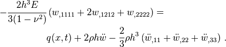
The governing equations simplify considerably for isotropic and homogeneous plates for which the in-plane deformations can be neglected. In that case we are left with one equation of the following form (in rectangular Cartesian coordinates):
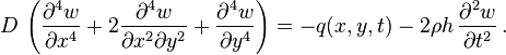
where  is the bending stiffness of the plate. For a uniform plate of thickness ,
In direct notation

For free vibrations, the governing equation becomes
Derivation of dynamic governing equations for isotropic Kirchhoff-Love plates For an isotropic and homogeneous plate, the stress-strain relations are
where
 are the in-plane strains. The strain-displacement relations
for Kirchhoff-Love plates are
are the in-plane strains. The strain-displacement relations
for Kirchhoff-Love plates areTherefore, the resultant moments corresponding to these stresses are
The governing equation for an isotropic and homogeneous plate of uniform thickness
in the
absence of in-plane displacements isDifferentiation of the expressions for the moment resultants gives us
Plugging into the governing equations leads to
Since the order of differentiation is irrelevant we have
 . Hence
If the flexural stiffness of the plate is defined as
we have
For small deformations, we often neglect the spatial derivatives of the transverse acceleration of the plate and we are left with
Then, in direct tensor notation, the governing equation of the plate is


References
- ↑ A. E. H. Love, On the small free vibrations and deformations of elastic shells, Philosophical trans. of the Royal Society (London), 1888, Vol. série A, N° 17 p. 491–549.
- ↑ Reddy, J. N., 2007, Theory and analysis of elastic plates and shells, CRC Press, Taylor and Francis.
- ↑ 3.0 3.1 Timoshenko, S. and Woinowsky-Krieger, S., (1959), Theory of plates and shells, McGraw-Hill New York.