Killing vector field

A Killing vector field (red) with integral curves (blue) on a sphere.

In mathematics, a Killing vector field (often just Killing field), named after Wilhelm Killing, is a vector field on a Riemannian manifold (or pseudo-Riemannian manifold) that preserves the metric. Killing fields are the infinitesimal generators of isometries; that is, flows generated by Killing fields are continuous isometries of the manifold. More simply, the flow generates a symmetry, in the sense that moving each point on an object the same distance in the direction of the Killing vector field will not distort distances on the object.

Definition

Specifically, a vector field X is a Killing field if the Lie derivative with respect to X of the metric g vanishes:

\mathcal{L}_{X} g = 0 \,.

In terms of the Levi-Civita connection, this is

g(\nabla_{Y} X, Z) + g(Y, \nabla_{Z} X) = 0 \,

for all vectors Y and Z. In local coordinates, this amounts to the Killing equation

\nabla_{\mu} X_{\nu} + \nabla_{\nu} X_{\mu} = 0 \,.

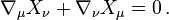
This condition is expressed in covariant form. Therefore it is sufficient to establish it in a preferred coordinate system in order to have it hold in all coordinate systems.

Examples

The vector field on a circle that points clockwise and has the same length at each point is a Killing vector field, since moving each point on the circle along this vector field simply rotates the circle.

If the metric coefficients $g_{\mu \nu} \,$ in some coordinate basis $dx^{a} \,$ are independent of $x^{\kappa} \,$ , then $K^{\mu} = \delta^{\mu}_{\kappa} \,$ is automatically a Killing vector, where $\delta^{\mu}_{\kappa} \,$ is the Kronecker delta.^[1]
To prove this, let us assume $g_{\mu \nu},_0=0 \,$
Then $K^\mu=\delta^{\mu}_{0} \,$ and $K_{\mu}=g_{\mu \nu} K^{\nu}= g_{\mu \nu} \delta^{\nu}_{0}= g_{\mu 0} \,$
Now let us look at the Killing condition
$K_{\mu;\nu}+K_{\nu;\mu}=K_{\mu,\nu}+K_{\nu,\mu}-2\Gamma^{\rho}_{\mu\nu}K_{\rho} = g_{\mu 0,\nu}+g_{\nu 0,\mu}-g^{\rho\sigma}(g_{\sigma\mu,\nu}+g_{\sigma\nu,\mu}-g_{\mu\nu,\sigma})g_{\rho 0} \,$
and from $g_{\rho 0}g^{\rho \sigma} = \delta_{0}^{\sigma} \,$
The Killing condition becomes
$g_{\mu 0,\nu}+g_{\nu 0,\mu} - ( g_{0\mu,\nu}+g_{0\nu,\mu}-g_{\mu\nu,0} ) = 0 \,$
that is $g_{\mu\nu,0}= 0$ , which is true.
The physical meaning is, for example, that, if none of the metric coefficients is a function of time, the manifold must automatically have a time-like Killing vector.

In layman's terms, if an object doesn't transform or "evolve" in time (when time passes), time passing won't change the measures of the object. Formulated like this, the result sounds like a tautology, but one has to understand that the example is very much contrived: Killing fields apply also to much more complex and interesting cases.

Properties

A Killing field is determined uniquely by a vector at some point and its gradient (i.e. all covariant derivatives of the field at the point).

The Lie bracket of two Killing fields is still a Killing field. The Killing fields on a manifold M thus form a Lie subalgebra of vector fields on M. This is the Lie algebra of the isometry group of the manifold if M is complete.

For compact manifolds

Negative Ricci curvature implies there are no nontrivial (nonzero) Killing fields.
Nonpositive Ricci curvature implies that any Killing field is parallel. i.e. covariant derivative along any vector j field is identically zero.
If the sectional curvature is positive and the dimension of M is even, a Killing field must have a zero.

The divergence of every Killing vector field vanishes.

If $X$ is a Killing vector field and $Y$ is a harmonic vector field, then $g(X,Y)$ is a harmonic function.

If $X$ is a Killing vector field and $\omega$ is a harmonic p-form, then $\mathcal{L}_{X} \omega = 0 \,.$

Geodesics

Each Killing vector corresponds to a quantity which is conserved along geodesics. This conserved quantity is the metric product between the Killing vector and the geodesic tangent vector. That is, along a geodesic with some affine parameter $\lambda$ , the equation 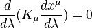$\frac d {d\lambda} ( K_\mu \frac{dx^\mu}{d\lambda} ) = 0$ is satisfied. This aids in analytically studying motions in a spacetime with symmetries.^[2]

Generalizations

Killing vector fields can be generalized to conformal Killing vector fields defined by $\mathcal{L}_{X} g = \lambda g \,$ for some scalar $\lambda \,.$ The derivatives of one parameter families of conformal maps are conformal Killing fields.
Killing tensor fields are symmetric tensor fields T such that the trace-free part of the symmetrization of $\nabla T \,$ vanishes. Examples of manifolds with Killing tensors include the rotating black hole and the FRW cosmology.^[3]
Killing vector fields can also be defined on any (possibly nonmetric) manifold M if we take any Lie group G acting on it instead of the group of isometries.^[4] In this broader sense, a Killing vector field is the pushforward of a right invariant vector field on G by the group action. If the group action is effective, then the space of the Killing vector fields is isomorphic to the Lie algebra $\mathfrak{g}$ of G.

Notes

↑ Misner, Thorne, Wheeler (1973). Gravitation. W H Freeman and Company. ISBN 0-7167-0344-0.
↑ Carrol, Sean (2004). An Introduction to General Relativity Spacetime and Geometry. Addison Wesley. pp. 133–139.
↑ Carrol, Sean (2004). An Introduction to General Relativity Spacetime and Geometry. Addison Wesley. pp. 263,344.
↑ Choquet-Bruhat, Yvonne; DeWitt-Morette, Cécile (1977), Analysis, Manifolds and Physics, Amsterdam: Elsevier, ISBN 978-0-7204-0494-4

References

Jost, Jurgen (2002). Riemannian Geometry and Geometric Analysis. Berlin: Springer-Verlag. ISBN 3-540-42627-2. .
Adler, Ronald; Bazin, Maurice & Schiffer, Menahem (1975). Introduction to General Relativity (Second Edition). New York: McGraw-Hill. ISBN 0-07-000423-4. . See chapters 3,9