Kernel regression
- Not to be confused with Kernel principal component analysis.
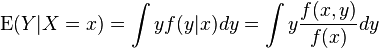
The kernel regression is a non-parametric technique in statistics to estimate the conditional expectation of a random variable. The objective is to find a non-linear relation between a pair of random variables X and Y.
In any nonparametric regression, the conditional expectation of a variable  relative to a variable
  may be written:

where  is an unknown function.
Nadaraya-Watson kernel regression
Nadaraya 1964 and Watson 1964 proposed to estimate as a locally weighted average, using a kernel as a weighting function. The Nadaraya-Watson estimator is:
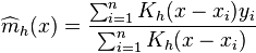
where  is a kernel with a bandwidth
  . The fraction is a weighting term with sum 1.
Derivation
Using the kernel density estimation for the joint distribution f(x,y) and f(x) with a kernel K,
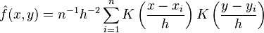 ,
,
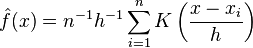
we obtain the Nadaraya-Watson estimator.
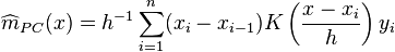
Priestley-Chao kernel estimator
Gasser-Müller kernel estimator
![\widehat{m}_{GM}(x) = h^{-1} \sum_{i=1}^n \left[\int_{s_{i-1}}^{s_i} K\left(\frac{x-u}{h}\right) du\right] y_i](../I/m/9efb47c3c8770b0b974512e124a80a28.png)
where 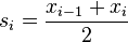
Example
This example is based upon Canadian cross-section wage data consisting of a random sample taken from the 1971 Canadian Census Public Use Tapes for male individuals having common education (grade 13). There are 205 observations in total.
We consider estimating the unknown regression function using Nadaraya-Watson kernel regression via the R np package that uses automatic (data-driven) bandwidth selection; see the np vignette for an introduction to the np package.
The figure below shows the estimated regression function using a second order Gaussian kernel along with asymptotic variability bounds

Script for example
The following commands of the R programming language use the npreg() function to deliver optimal smoothing and to create The the figure given above. These commands can be entered at the command prompt via cut and paste.
install.packages("np")
library(np) # non parametric library
data(cps71)
attach(cps71)

m <- npreg(logwage~age)

plot(m,plot.errors.method="asymptotic",
     plot.errors.style="band",
     ylim=c(11,15.2))

points(age,logwage,cex=.25)
Related
According to Salsburg 2002, pp. 290–1, the algorithms used in kernel regression were independently developed and used in fuzzy systems: "Coming up with almost exactly the same computer algorithm, fuzzy systems and kernel density-based regressions appear to have been developed completely independently of one another."
References
- Nadaraya, E. A. (1964). "On Estimating Regression". Theory of Probability and its Applications 9 (1): 141–2. doi:10.1137/1109020.
- Li, Qi; Racine, Jeffrey S. (2007). Nonparametric Econometrics: Theory and Practice. Princeton University Press. ISBN 0-691-12161-3.
- Simonoff, Jeffrey S. (1996). Smoothing Methods in Statistics. Springer. ISBN 0-387-94716-7.
- Salsburg, D. (2002). The Lady Tasting Tea: How Statistics Revolutionized Science in the Twentieth Century. W.H. Freeman. ISBN 0-8050-7134-2.
- Richard, C.; Bermudez, J.-C. M.; Honeine, P. (March 2009). "Online prediction of time series data with kernels" (PDF). IEEE Transactions on Signal Processing 57 (3): 1058–67. doi:10.1109/TSP.2008.2009895.
- Parreira, W.; Bermudez, J.-C. M.; Richard, C.; Tourneret, J.-Y. (May 2012). "Stochastic behavior analysis of the Gaussian kernel-least-mean-square algorithm." (PDF). IEEE Transactions on Signal Processing 60 (5): 2208–2222. doi:10.1109/TSP.2012.2186132.
- Richard, C.; Bermudez, J.-C. M. (November 2012). "Closed-form conditions for convergence of the Gaussian kernel-least-mean-square algorithm." (PDF). Proc. of Asilomar'12: 1797–1801. doi:10.1109/ACSSC.2012.6489344.
- Watson, G. S. (1964). "Smooth regression analysis". Sankhyā: The Indian Journal of Statistics, Series A 26 (4): 359–372. JSTOR 25049340.
- Fan, J. (1993) "Local linear regression smoothers and their minimax efficiency" Ann. Statist., 21, pp. 196–216
- Fan, J. and I. Gijbels (1992) Variable bandwidth and local linear regression smoothers, Ann. Statist., 20, pp. 2008–2036
- Fan, J. and I. Gijbels (1996) Local Polynomial Modelling and its Applications, Chapman and Hall
- Li, Q. and J. Racine (2007) Nonparametric Econometrics: Theory and Practice, Princeton University Press
- Li, D., Simar, L. and V. Zelenyuk (2014) "Generalized nonparametric smoothing with mixed discrete and continuous data" Computational Statistics and Data Analysis, 1-21. doi:10.1016/j.csda.2014.06.003
- Pagan, A. and A. Ullah (1999) Nonparametric Econometrics, Cambridge University Press.
- Racine, J. and Q. Li, (2004) "Nonparametric estimation of regression functions with both categorical and continuous data" Journal of Econometrics 119, pp. 99–130
- Park, Byeong U. & Simar, Léopold & Zelenyuk, Valentin, 2008. "Local likelihood estimation of truncated regression and its partial derivatives: Theory and application," Journal of Econometrics, Elsevier, vol. 146(1), pages 185-198, September.
Statistical implementation
kernreg2 y x, bwidth(.5) kercode(3) npoint(500) gen(kernelprediction gridofpoints)
- R: npreg (package np)
- GNU/octave mathematical program package:
External links
- Scale-adaptive kernel regression (with Matlab software).
- Tutorial of Kernel regression using spreadsheet (with Microsoft Excel).
- An online kernel regression demonstration Requires .NET 3.0 or later.
- The np package An R package that provides a variety of nonparametric and semiparametric kernel methods that seamlessly handle a mix of continuous, unordered, and ordered factor data types.