Kernel density estimation
In statistics, kernel density estimation (KDE) is a non-parametric way to estimate the probability density function of a random variable. Kernel density estimation is a fundamental data smoothing problem where inferences about the population are made, based on a finite data sample. In some fields such as signal processing and econometrics it is also termed the Parzen–Rosenblatt window method, after Emanuel Parzen and Murray Rosenblatt, who are usually credited with independently creating it in its current form.[1][2]
Definition
Let (x1, x2, …, xn) be an independent and identically distributed sample drawn from some distribution with an unknown density ƒ. We are interested in estimating the shape of this function ƒ. Its kernel density estimator is
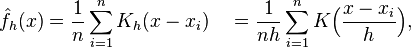
where K(•) is the kernel — a non-negative function that integrates to one and has mean zero — and h > 0 is a smoothing parameter called the bandwidth. A kernel with subscript h is called the scaled kernel and defined as Kh(x) = 1/h K(x/h). Intuitively one wants to choose h as small as the data allow, however there is always a trade-off between the bias of the estimator and its variance; more on the choice of bandwidth below.
A range of kernel functions are commonly used: uniform, triangular, biweight, triweight, Epanechnikov, normal, and others. The Epanechnikov kernel is optimal in a mean square error sense,[3] though the loss of efficiency is small for the kernels listed previously,[4] and due to its convenient mathematical properties, the normal kernel is often used K(x) = ϕ(x), where ϕ is the standard normal density function.
The construction of a kernel density estimate finds interpretations in fields outside of density estimation. For example, in thermodynamics, this is equivalent to the amount of heat generated when heat kernels (the fundamental solution to the heat equation) are placed at each data point locations xi. Similar methods are used to construct discrete Laplace operators on point clouds for manifold learning.
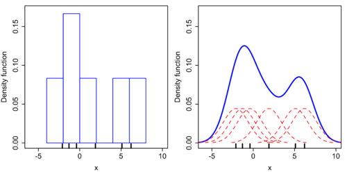
Kernel density estimates are closely related to histograms, but can be endowed with properties such as smoothness or continuity by using a suitable kernel. To see this, we compare the construction of histogram and kernel density estimators, using these 6 data points: x1 = −2.1, x2 = −1.3, x3 = −0.4, x4 = 1.9, x5 = 5.1, x6 = 6.2. For the histogram, first the horizontal axis is divided into sub-intervals or bins which cover the range of the data. In this case, we have 6 bins each of width 2. Whenever a data point falls inside this interval, we place a box of height 1/12. If more than one data point falls inside the same bin, we stack the boxes on top of each other.
For the kernel density estimate, we place a normal kernel with variance 2.25 (indicated by the red dashed lines) on each of the data points xi. The kernels are summed to make the kernel density estimate (solid blue curve). The smoothness of the kernel density estimate is evident compared to the discreteness of the histogram, as kernel density estimates converge faster to the true underlying density for continuous random variables.[5]
Bandwidth selection
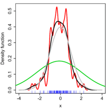
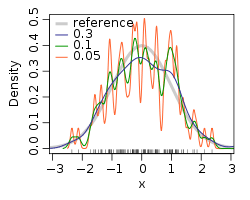
The bandwidth of the kernel is a free parameter which exhibits a strong influence on the resulting estimate. To illustrate its effect, we take a simulated random sample from the standard normal distribution (plotted at the blue spikes in the rug plot on the horizontal axis). The grey curve is the true density (a normal density with mean 0 and variance 1). In comparison, the red curve is undersmoothed since it contains too many spurious data artifacts arising from using a bandwidth h = 0.05, which is too small. The green curve is oversmoothed since using the bandwidth h = 2 obscures much of the underlying structure. The black curve with a bandwidth of h = 0.337 is considered to be optimally smoothed since its density estimate is close to the true density.
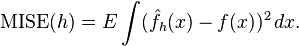
The most common optimality criterion used to select this parameter is the expected L2 risk function, also termed the mean integrated squared error:
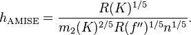
Under weak assumptions on ƒ and K,[1][2] MISE (h) = AMISE(h) + o(1/(nh) + h4) where o is the little o notation. The AMISE is the Asymptotic MISE which consists of the two leading terms
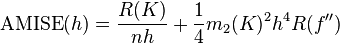
where 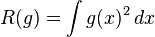 for a function g,
  and ƒ'' is the second derivative of ƒ. The minimum of this AMISE is the solution to this differential equation
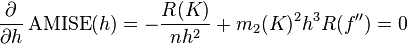
or
Neither the AMISE nor the hAMISE formulas are able to be used directly since they involve the unknown density function ƒ or its second derivative ƒ'', so a variety of automatic, data-based methods have been developed for selecting the bandwidth. Many review studies have been carried out to compare their efficacities,[6][7][8][9][10] with the general consensus that the plug-in selectors[11] and cross validation selectors[12][13][14] are the most useful over a wide range of data sets.
Substituting any bandwidth h which has the same asymptotic order n−1/5 as hAMISE into the AMISE gives that AMISE(h) = O(n−4/5), where O is the big o notation. It can be shown that, under weak assumptions, there cannot exist a non-parametric estimator that converges at a faster rate than the kernel estimator.[15] Note that the n−4/5 rate is slower than the typical n−1 convergence rate of parametric methods.
If the bandwidth is not held fixed, but is varied depending upon the location of either the estimate (balloon estimator) or the samples (pointwise estimator), this produces a particularly powerful method termed adaptive or variable bandwidth kernel density estimation.
Practical estimation of the bandwidth
If Gaussian basis functions are used to approximate univariate data, and the underlying density being estimated is Gaussian then it can be shown that the optimal choice for h is[16]
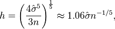
where  is the standard deviation of the samples.
This approximation is termed the normal distribution approximation, Gaussian approximation, or Silverman's rule of thumb.
is the standard deviation of the samples.
This approximation is termed the normal distribution approximation, Gaussian approximation, or Silverman's rule of thumb.
Relation to the characteristic function density estimator
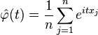
Given the sample (x1, x2, …, xn), it is natural to estimate the characteristic function φ(t) = E[eitX] as
Knowing the characteristic function, it is possible to find the corresponding probability density function through the Fourier transform formula. One difficulty with applying this inversion formula is that it leads to a diverging integral, since the estimate  is unreliable for large t’s. To circumvent this problem, the estimator is multiplied by a damping function ψh(t) = ψ(ht), which is equal to 1 at the origin and then falls to 0 at infinity. The “bandwidth parameter” h controls how fast we try to dampen the function . In particular when h is small, then ψh(t) will be approximately one for a large range of t’s, which means that remains practically unaltered in the most important region of t’s.
The most common choice for function ψ is either the uniform function ψ(t) = 1{−1 ≤ t ≤ 1}, which effectively means truncating the interval of integration in the inversion formula to [−1/h, 1/h], or the gaussian function ψ(t) = e−π t2. Once the function ψ has been chosen, the inversion formula may be applied, and the density estimator will be
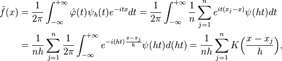
where K is the Fourier transform of the damping function ψ. Thus the kernel density estimator coincides with the characteristic function density estimator.
Statistical implementation
A non-exhaustive list of software implementations of kernel density estimators includes:
- In Analytica release 4.4, the Smoothing option for PDF results uses KDE, and from expressions it is available via the built-in
Pdffunction. - In C/C++, FIGTree is a library that can be used to compute kernel density estimates using normal kernels. MATLAB interface available.
- In C++, libagf is a library for variable kernel density estimation.
- In CrimeStat, kernel density estimation is implemented using five different kernel functions – normal, uniform, quartic, negative exponential, and triangular. Both single- and dual-kernel density estimate routines are available. Kernel density estimation is also used in interpolating a Head Bang routine, in estimating a two-dimensional Journey-to-crime density function, and in estimating a three-dimensional Bayesian Journey-to-crime estimate.
- In ELKI, kernel density functions can be found in the package
de.lmu.ifi.dbs.elki.math.statistics.kernelfunctions - In ESRI products, kernel density mapping is managed out of the Spatial Analyst toolbox and uses the Quartic(biweight) kernel.
- In Excel, the Royal Society of Chemistry has created an add-in to run kernel density estimation based on their Analytical Methods Committee Technical Brief 4.
- In gnuplot, kernel density estimation is implemented by the
smooth kdensityoption, the datafile can contain a weight and bandwidth for each point, or the bandwidth can be set automatically[17] according to "Silverman's rule of thumb" (see above). - In Haskell, kernel density is implemented in the statistics package.
- In Java, the Weka (machine learning) package provides weka.estimators.KernelEstimator, among others.
- In JavaScript, the visualization package D3.js offers a KDE package in its science.stats package.
- In JMP, The Distribution platform can be used to create univariate kernel density estimates, and the Fit Y by X platform can be used to create bivariate kernel density estimates.
- In Julia, kernel density estimation is implemented in the KernelDensity.jl package.
- In MATLAB, kernel density estimation is implemented through the
ksdensityfunction (Statistics Toolbox). This function does not provide an automatic data-driven bandwidth but uses a rule of thumb, which is optimal only when the target density is normal. A free MATLAB software package which implements an automatic bandwidth selection method[18] is available from the MATLAB Central File Exchange for 1-dimensional data and for 2-dimensional data. - In Mathematica, numeric kernel density estimation is implemented by the function
SmoothKernelDistributionhere and symbolic estimation is implemented using the functionKernelMixtureDistributionhere both of which provide data-driven bandwidths. - In Minitab, the Royal Society of Chemistry has created a macro to run kernel density estimation based on their Analytical Methods Committee Technical Brief 4.
- In the NAG Library, kernel density estimation is implemented via the
g10baroutine (available in both the Fortran[19] and the C[20] versions of the Library). - In Octave, kernel density estimation is implemented by the
kernel_densityoption (econometrics package). - In Origin, 2D kernel density plot can be made from its user interface, and two functions, Ksdensity for 1D and Ks2density for 2D can be used from its LabTalk, Python, or C code.
- In Perl, an implementation can be found in the Statistics-KernelEstimation module
- In Python, many implementations exist: SciPy (
scipy.stats.gaussian_kde), Statsmodels (KDEUnivariateandKDEMultivariate), and Scikit-learn (KernelDensity) (see comparison[21]).
- In R, it is implemented through the
densityand thebkdefunction in the KernSmooth library (both included in the base distribution), thekdefunction in the ks library, thedkdenanddbckdenfunctions in the evmix library (latter for boundary corrected kernel density estimation for bounded support), thenpudensfunction in the np library (numeric and categorical data), thesm.densityfunction in the sm library. For an implementation of thekde.Rfunction, which does not require installing any packages or libraries, see kde.R. - In SAS,
proc kdecan be used to estimate univariate and bivariate kernel densities. - In Stata, it is implemented through
kdensity; for examplehistogram x, kdensity. Alternatively a free Stata module KDENS is available from here allowing a user to estimate 1D or 2D density functions.
Examples
Example in MATLAB-Octave
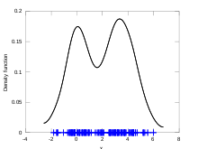
For this example, the data are a synthetic sample of 50 points drawn from the standard normal and 50 points from a normal distribution with mean 3.5 and variance 1. The automatic bandwidth selection and density estimation with normal kernels is carried out by kde.m. This function implements an automatic bandwidth selector that does not rely on the commonly used Gaussian plug-in rule of thumb heuristic.[18]
 randn('seed',8192);
 x = [randn(50,1); randn(50,1)+3.5];
 [h, fhat, xgrid] = kde(x, 401);
 figure;
 hold on;
 plot(xgrid, fhat, 'linewidth', 2, 'color', 'black');
 plot(x, zeros(100,1), 'b+');
 xlabel('x')
 ylabel('Density function')
 hold off;
Example in R
_KDE_with_plugin_bandwidth.png)
This example is based on the Old Faithful Geyser, a tourist attraction located in Yellowstone National Park. This famous dataset containing 272 records consists of two variables, eruption duration, and waiting time until next eruption, both in minutes, included in the base distribution of R. We analyse the waiting times, using the ks library since it has a wide range of visualisation options. The bandwidth function is hpi which in turn calls the dpik function in the KernSmooth library: these functions implement the plug-in selector.[11] The kernel density estimate using the normal kernel is computed using kde which calls bkde from KernSmooth. The plot function allows the addition of the data points as a rug plot on the horizontal axis. The bimodal structure in the density estimate of the waiting times is clearly seen, in contrast to the rug plot where this structure is not apparent.
 library(KernSmooth)
 attach(faithful)
 fhat <- bkde(x=waiting)
 plot (fhat, xlab="x", ylab="Density function")
Example in Python
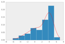
To demonstrate how kernel density estimation is performed in Python, we simulate some data from a mixture of normals, where 50 observations are generated from a normal distribution with mean zero and standard deviation 3 and another 50 from a normal with mean 4 and standard deviation 1.
import numpy as np

x1 = np.random.normal(0, 3, 50)
x2 = np.random.normal(4, 1, 50)
x = np.r_[x1, x2]
The gaussian_kde function from the SciPy package implements a kernel-density estimate using Gaussian kernels, and includes automatic determination of bandwidth. By default, gaussian_kde uses Scott's rule to select the appropriate bandwidth.[22]
from scipy.stats import kde
import matplotlib.pyplot as plt

density = kde.gaussian_kde(x)
xgrid = np.linspace(x.min(), x.max(), 100)
plt.hist(x, bins=8, normed=True)
plt.plot(xgrid, density(xgrid), 'r-')
plt.show()
The plot shows both a histogram of the simulated data, along with a red line that shows the Gaussian KDE.
See also
| Wikimedia Commons has media related to Kernel density estimation. |
- Kernel (statistics)
- Kernel smoothing
- Kernel regression
- Density estimation (with presentation of other examples)
- Mean-shift
- Scale space The triplets {(x, h, KDE with bandwidth h evaluated at x: all x, h > 0} form a scale space representation of the data.
- Multivariate kernel density estimation
- Variable kernel density estimation
References
- ↑ 1.0 1.1 Rosenblatt, M. (1956). "Remarks on Some Nonparametric Estimates of a Density Function". The Annals of Mathematical Statistics 27 (3): 832. doi:10.1214/aoms/1177728190.
- ↑ 2.0 2.1 Parzen, E. (1962). "On Estimation of a Probability Density Function and Mode". The Annals of Mathematical Statistics 33 (3): 1065. doi:10.1214/aoms/1177704472. JSTOR 2237880.
- ↑ Epanechnikov, V.A. (1969). "Non-parametric estimation of a multivariate probability density". Theory of Probability and its Applications 14: 153–158. doi:10.1137/1114019.
- ↑ Wand, M.P; Jones, M.C. (1995). Kernel Smoothing. London: Chapman & Hall/CRC. ISBN 0-412-55270-1.
- ↑ Scott, D. (1979). "On optimal and data-based histograms". Biometrika 66 (3): 605–610. doi:10.1093/biomet/66.3.605.
- ↑ Park, B.U.; Marron, J.S. (1990). "Comparison of data-driven bandwidth selectors". Journal of the American Statistical Association 85 (409): 66–72. doi:10.1080/01621459.1990.10475307. JSTOR 2289526.
- ↑ Park, B.U.; Turlach, B.A. (1992). "Practical performance of several data driven bandwidth selectors (with discussion)". Computational Statistics 7: 251–270.
- ↑ Cao, R.; Cuevas, A.; Manteiga, W. G. (1994). "A comparative study of several smoothing methods in density estimation". Computational Statistics and Data Analysis 17 (2): 153–176. doi:10.1016/0167-9473(92)00066-Z.
- ↑ Jones, M.C.; Marron, J.S.; Sheather, S. J. (1996). "A brief survey of bandwidth selection for density estimation". Journal of the American Statistical Association 91 (433): 401–407. doi:10.2307/2291420. JSTOR 2291420.
- ↑ Sheather, S.J. (1992). "The performance of six popular bandwidth selection methods on some real data sets (with discussion)". Computational Statistics 7: 225–250, 271–281.
- ↑ 11.0 11.1 Sheather, S.J.; Jones, M.C. (1991). "A reliable data-based bandwidth selection method for kernel density estimation". Journal of the Royal Statistical Society, Series B 53 (3): 683–690. JSTOR 2345597.
- ↑ Rudemo, M. (1982). "Empirical choice of histograms and kernel density estimators". Scandinavian Journal of Statistics 9 (2): 65–78. JSTOR 4615859.
- ↑ Bowman, A.W. (1984). "An alternative method of cross-validation for the smoothing of density estimates". Biometrika 71 (2): 353–360. doi:10.1093/biomet/71.2.353.
- ↑ Hall, P.; Marron, J.S.; Park, B.U. (1992). "Smoothed cross-validation". Probability Theory and Related Fields 92: 1–20. doi:10.1007/BF01205233.
- ↑ Wahba, G. (1975). "Optimal convergence properties of variable knot, kernel, and orthogonal series methods for density estimation". Annals of Statistics 3 (1): 15–29. doi:10.1214/aos/1176342997.
- ↑ Silverman, B.W. (1998). Density Estimation for Statistics and Data Analysis. London: Chapman & Hall/CRC. p. 48. ISBN 0-412-24620-1.
- ↑ Janert, Philipp K (2009). Gnuplot in action : understanding data with graphs. Connecticut, USA: Manning Publications. ISBN 978-1-933988-39-9. See section 13.2.2 entitled Kernel density estimates.
- ↑ 18.0 18.1 Botev, Z.I.; Grotowski, J.F.; Kroese, D.P. (2010). "Kernel density estimation via diffusion". Annals of Statistics 38 (5): 2916–2957. doi:10.1214/10-AOS799.
- ↑ The Numerical Algorithms Group. "NAG Library Routine Document: nagf_smooth_kerndens_gauss (g10baf)". NAG Library Manual, Mark 23. Retrieved 2012-02-16.
- ↑ The Numerical Algorithms Group. "NAG Library Routine Document: nag_kernel_density_estim (g10bac)". NAG Library Manual, Mark 9. Retrieved 2012-02-16.
- ↑ Vanderplas, Jake (2013-12-01). "Kernel Density Estimation in Python". Retrieved 2014-03-12.
- ↑ scipy.stats.gaussian_kde, SciPy.org
External links
- Introduction to kernel density estimation A short tutorial which motivates kernel density estimators as an improvement over histograms.
- Kernel Bandwidth Optimization A free online tool that instantly generates an optimized kernel density estimate of your data.
- Free Online Software (Calculator) computes the Kernel Density Estimation for any data series according to the following Kernels: Gaussian, Epanechnikov, Rectangular, Triangular, Biweight, Cosine, and Optcosine.
- Kernel Density Estimation Applet An online interactive example of kernel density estimation. Requires .NET 3.0 or later.