Jacobi method
In numerical linear algebra, the Jacobi method (or Jacobi iterative method[1]) is an algorithm for determining the solutions of a diagonally dominant system of linear equations. Each diagonal element is solved for, and an approximate value is plugged in. The process is then iterated until it converges. This algorithm is a stripped-down version of the Jacobi transformation method of matrix diagonalization. The method is named after Carl Gustav Jacob Jacobi.
Description
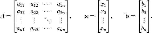
Given a square system of n linear equations:

where:
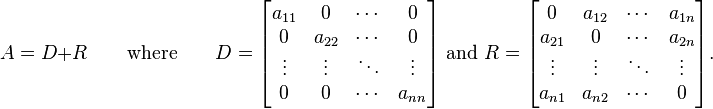
Then A can be decomposed into a diagonal component D, and the remainder R:
The solution is then obtained iteratively via
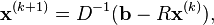
where  is the kth approximation or iteration of
  and
and  is the next or k + 1 iteration of .
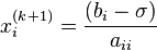
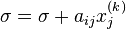
The element-based formula is thus:
is the next or k + 1 iteration of .
The element-based formula is thus:
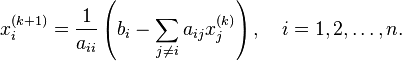
The computation of xi(k+1) requires each element in x(k) except itself. Unlike the Gauss–Seidel method, we can't overwrite xi(k) with xi(k+1), as that value will be needed by the rest of the computation. The minimum amount of storage is two vectors of size n.
Algorithm
- Choose an initial guess
 to the solution
 -

- while convergence not reached do
- for i := 1 step until n do
-

- for j := 1 step until n do
- if j ≠ i then
-
- end if
- if j ≠ i then
- end (j-loop)
-
-
- end (i-loop)
- check if convergence is reached
-

- for i := 1 step until n do
- loop (while convergence condition not reached)
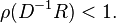
Convergence
The standard convergence condition (for any iterative method) is when the spectral radius of the iteration matrix is less than 1:
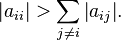
The method is guaranteed to converge if the matrix A is strictly or irreducibly diagonally dominant. Strict row diagonal dominance means that for each row, the absolute value of the diagonal term is greater than the sum of absolute values of other terms:
The Jacobi method sometimes converges even if these conditions are not satisfied.
Example
A linear system of the form  with initial estimate is given by
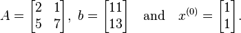
We use the equation 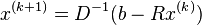 , described above, to estimate
  . First, we rewrite the equation in a more convenient form
 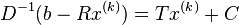 , where
 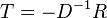 and
and  . Note that
  where
where  and
and  are the strictly lower and upper parts of
  . From the known values
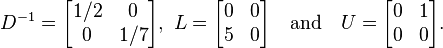
we determine 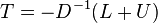 as
as

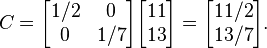
Further, C is found as
With T and C calculated, we estimate as 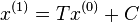 :
:
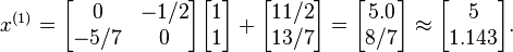
The next iteration yields

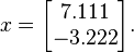
This process is repeated until convergence (i.e., until  is small). The solution after 25 iterations is
Another example
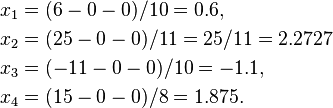
Suppose we are given the following linear system:
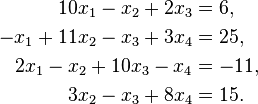
Suppose we choose (0, 0, 0, 0) as the initial approximation, then the first approximate solution is given by
Using the approximations obtained, the iterative procedure is repeated until the desired accuracy has been reached. The following are the approximated solutions after five iterations.
 |
 |
 |
 |
|---|---|---|---|
 |
 |
 |
 |
 |
 |
 |
 |
 |
 |
 |
 |
 |
 |
 |
 |
 |
 |
 |
 |
The exact solution of the system is (1, 2, −1, 1).
An example using Python 3 and Numpy
The following numerical procedure simply iterates to produce the solution vector.
import numpy as np

ITERATION_LIMIT = 1000

# initialize the matrix
A = np.array([[10., -1., 2., 0.],
              [-1., 11., -1., 3.],
              [2., -1., 10., -1.],
              [0.0, 3., -1., 8.]])
# initialize the RHS vector
b = np.array([6., 25., -11., 15.])

# prints the system
print("System:")
for i in range(A.shape[0]):
    row = ["{}*x{}".format(A[i, j], j + 1) for j in range(A.shape[1])]
    print(" + ".join(row), "=", b[i])
print()

x = np.zeros_like(b)
for it_count in range(ITERATION_LIMIT):
    print("Current solution:", x)
    x_new = np.zeros_like(x)

    for i in range(A.shape[0]):
        s1 = np.dot(A[i, :i], x[:i])
        s2 = np.dot(A[i, i + 1:], x[i + 1:])
        x_new[i] = (b[i] - s1 - s2) / A[i, i]

    if np.allclose(x, x_new, atol=1e-10):
        break

    x = x_new

print("Solution:")
print(x)
error = np.dot(A, x) - b
print("Error:")
print(error)
Produces the output:
System:
10.0*x1 + -1.0*x2 + 2.0*x3 + 0.0*x4 = 6.0
-1.0*x1 + 11.0*x2 + -1.0*x3 + 3.0*x4 = 25.0
2.0*x1 + -1.0*x2 + 10.0*x3 + -1.0*x4 = -11.0
0.0*x1 + 3.0*x2 + -1.0*x3 + 8.0*x4 = 15.0

Current solution: [ 0.  0.  0.  0.]
Current solution: [ 0.6         2.27272727 -1.1         1.875     ]
Current solution: [ 1.04727273  1.71590909 -0.80522727  0.88522727]
Current solution: [ 0.93263636  2.05330579 -1.04934091  1.13088068]
Current solution: [ 1.01519876  1.95369576 -0.96810863  0.97384272]
Current solution: [ 0.9889913   2.01141473 -1.0102859   1.02135051]
Current solution: [ 1.00319865  1.99224126 -0.99452174  0.99443374]
Current solution: [ 0.99812847  2.00230688 -1.00197223  1.00359431]
Current solution: [ 1.00062513  1.9986703  -0.99903558  0.99888839]
Current solution: [ 0.99967415  2.00044767 -1.00036916  1.00061919]
Current solution: [ 1.0001186   1.99976795 -0.99982814  0.99978598]
Current solution: [ 0.99994242  2.00008477 -1.00006833  1.0001085 ]
Current solution: [ 1.00002214  1.99995896 -0.99996916  0.99995967]
Current solution: [ 0.99998973  2.00001582 -1.00001257  1.00001924]
Current solution: [ 1.00000409  1.99999268 -0.99999444  0.9999925 ]
Current solution: [ 0.99999816  2.00000292 -1.0000023   1.00000344]
Current solution: [ 1.00000075  1.99999868 -0.99999899  0.99999862]
Current solution: [ 0.99999967  2.00000054 -1.00000042  1.00000062]
Current solution: [ 1.00000014  1.99999976 -0.99999982  0.99999975]
Current solution: [ 0.99999994  2.0000001  -1.00000008  1.00000011]
Current solution: [ 1.00000003  1.99999996 -0.99999997  0.99999995]
Current solution: [ 0.99999999  2.00000002 -1.00000001  1.00000002]
Current solution: [ 1.          1.99999999 -0.99999999  0.99999999]
Current solution: [ 1.  2. -1.  1.]
Solution:
[ 1.  2. -1.  1.]
Error:
[ -2.81440107e-08   5.15706873e-08  -3.63466359e-08   4.17092547e-08]
Weighted Jacobi method
The weighted Jacobi iteration uses a parameter  to compute the iteration as

with  being the usual choice.[2]
Recent developments
In 2014, a refinement of the algorithm, called scheduled relaxation Jacobi method, was published.[1][3] The new method employs a schedule of over- and under-relaxations and provides a two-hundred fold performance improvement for solving elliptic equations discretized on large two- and three-dimensional Cartesian grids.
See also
- Gauss–Seidel method
- Successive over-relaxation
- Iterative method. Linear systems
- Gaussian Belief Propagation
- Matrix splitting
References
- ↑ 1.0 1.1 Johns Hopkins University (June 30, 2014). "19th century math tactic gets a makeover—and yields answers up to 200 times faster". Phys.org (Douglas, Isle Of Man, United Kingdom: Omicron Technology Limited). Retrieved 2014-07-01.
- ↑ Saad, Yousef (2003). Iterative Methods for Sparse Linear Systems (2 ed.). SIAM. p. 414. ISBN 0898715342.
- ↑ Yang, Xiang; Mittal, Rajat (June 27, 2014). "Acceleration of the Jacobi iterative method by factors exceeding 100 using scheduled relaxation". Journal of Computational Physics. doi:10.1016/j.jcp.2014.06.010.
External links
- Hazewinkel, Michiel, ed. (2001), "Jacobi method", Encyclopedia of Mathematics, Springer, ISBN 978-1-55608-010-4
- This article incorporates text from the article Jacobi_method on CFD-Wiki that is under the GFDL license.
- Black, Noel; Moore, Shirley; and Weisstein, Eric W., "Jacobi method", MathWorld.
- Jacobi Method from www.math-linux.com
- Module for Jacobi and Gauss–Seidel Iteration
- Numerical matrix inversion
| ||||||||||||||||||