Jacobi eigenvalue algorithm
In numerical linear algebra, the Jacobi eigenvalue algorithm is an iterative method for the calculation of the eigenvalues and eigenvectors of a real symmetric matrix (a process known as diagonalization). It is named after Carl Gustav Jacob Jacobi, who first proposed the method in 1846,[1] but only became widely used in the 1950s with the advent of computers.[2]
Description
Let S be a symmetric matrix, and G = G(i,j,θ) be a Givens rotation matrix. Then:

is symmetric and similar to S.
Furthermore, S′ has entries:
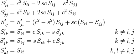
where s = sin(θ) and c = cos(θ).
Since G is orthogonal, S and S′ have the same Frobenius norm ||·||F (the square-root sum of squares of all components), however we can choose θ such that S′ij = 0, in which case S′ has a larger sum of squares on the diagonal:

Set this equal to 0, and rearrange:
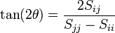
if 

In order to optimize this effect, Sij should be the off-diagonal component with the largest absolute value, called the pivot.
The Jacobi eigenvalue method repeatedly performs rotations until the matrix becomes almost diagonal. Then the elements in the diagonal are approximations of the (real) eigenvalues of S.
Convergence
If  is a pivot element, then by definition
  for
for  . Since S has exactly 2 N := n ( n - 1) off-diag elements, we have
 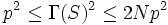 or
or 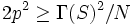 . This implies
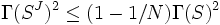 or
or 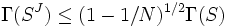 ,
i.e. the sequence of Jacobi rotations converges at least linearly by a factor
,
i.e. the sequence of Jacobi rotations converges at least linearly by a factor  to a diagonal matrix.
A number of N Jacobi rotations is called a sweep; let  denote the result. The previous estimate yields
-
 ,
,
i.e. the sequence of sweeps converges at least linearly with a factor ≈  .
.
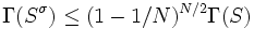
However the following result of Schönhage[3] yields locally quadratic convergence. To this end let S have m distinct eigenvalues  with multiplicities
  and let d > 0 be the smallest distance of two different eigenvalues. Let us call a number of
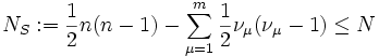
Jacobi rotations a Schönhage-sweep. If  denotes the result then
-
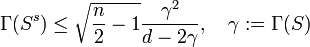 .
.
Thus convergence becomes quadratic as soon as 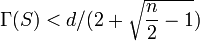
Cost
Each Jacobi rotation can be done in n steps when the pivot element p is known. However the search for p requires inspection of all N ≈ ½ n2 off-diag elements. We can reduce this to n steps too if we introduce an additional index array 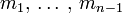 with the property that
  is the index of the largest element in row i, (i = 1, …, n − 1) of the current S. Then (k, l) must be one of the pairs
  . Since only columns k and l change, only
  must be updated, which again can be done in n steps. Thus each rotation has O(n) cost and one sweep has O(n3) cost which is equivalent to one matrix multiplication. Additionally the must be initialized before the process starts, this can be done in n2 steps.
Typically the Jacobi method converges within numerical precision after a small number of sweeps. Note that multiple eigenvalues reduce the number of iterations since  .
.
Algorithm
The following algorithm is a description of the Jacobi method in math-like notation.
It calculates a vector e which contains the eigenvalues and a matrix E which contains the corresponding eigenvectors, i.e.  is an eigenvalue and the column
  an orthonormal eigenvector for , i = 1, …, n.
procedure jacobi(S ∈ Rn×n; out e ∈ Rn; out E ∈ Rn×n)
  var
    i, k, l, m, state ∈ N
    s, c, t, p, y, d, r ∈ R
    ind ∈ Nn
    changed ∈ Ln

  function maxind(k ∈ N) ∈ N ! index of largest off-diagonal element in row k
    m := k+1
    for i := k+2 to n do
      if │Ski│ > │Skm│ then m := i endif
    endfor
    return m
  endfunc

  procedure update(k ∈ N; t ∈ R) ! update ek and its status
    y := ek; ek := y+t
    if changedk and (y=ek) then changedk := false; state := state−1
    elsif (not changedk) and (y≠ek) then changedk := true; state := state+1
    endif
  endproc

  procedure rotate(k,l,i,j ∈ N) ! perform rotation of Sij, Skl
    ┌   ┐    ┌     ┐┌   ┐
    │Skl│    │c  −s││Skl│
    │   │ := │     ││   │
    │Sij│    │s   c││Sij│
    └   ┘    └     ┘└   ┘
  endproc

  ! init e, E, and arrays ind, changed
  E := I; state := n
  for k := 1 to n do indk := maxind(k); ek := Skk; changedk := true endfor
  while state≠0 do ! next rotation
    m := 1 ! find index (k,l) of pivot p
    for k := 2 to n−1 do
      if │Sk indk│ > │Sm indm│ then m := k endif
    endfor
    k := m; l := indm; p := Skl
    ! calculate c = cos φ, s = sin φ
    y := (el−ek)/2; d := │y│+√(p2+y2)
    r := √(p2+d2); c := d/r; s := p/r; t := p2/d
    if y<0 then s := −s; t := −t endif
    Skl := 0.0; update(k,−t); update(l,t)
    ! rotate rows and columns k and l
    for i := 1 to k−1 do rotate(i,k,i,l) endfor
    for i := k+1 to l−1 do rotate(k,i,i,l) endfor
    for i := l+1 to n do rotate(k,i,l,i) endfor
    ! rotate eigenvectors
    for i := 1 to n do
      ┌   ┐    ┌     ┐┌   ┐
      │Eki│    │c  −s││Eki│
      │   │ := │     ││   │
      │Eli│    │s   c││Eli│
      └   ┘    └     ┘└   ┘
    endfor
    ! rows k, l have changed, update rows indk, indl
    indk := maxind(k); indl := maxind(l)
  loop
endproc
Notes
1. The logical array changed holds the status of each eigenvalue. If the numerical value of  or
or  changes during an iteration, the corresponding component of changed is set to true, otherwise to false. The integer state counts the number of components of changed which have the value true. Iteration stops as soon as state = 0. This means that none of the approximations
  has recently changed its value and thus it is not very likely that this will happen if iteration continues. Here it is assumed that floating point operations are optimally rounded to the nearest floating point number.
2. The upper triangle of the matrix S is destroyed while the lower triangle and the diagonal are unchanged. Thus it is possible to restore S if necessary according to
for k := 1 to n−1 do ! restore matrix S
  for l := k+1 to n do Skl := Slk endfor
endfor
3. The eigenvalues are not necessarily in descending order. This can be achieved by a simple sorting algorithm.
for k := 1 to n−1 do
  m := k
  for l := k+1 to n do
    if el > em then m := l endif
  endfor
  if k ≠ m then swap em,ek; swap Em,Ek endif
endfor
4. The algorithm is written using matrix notation (1 based arrays instead of 0 based).
5. When implementing the algorithm, the part specified using matrix notation must be performed simultaneously.
6. This implementation does not correctly account for the case in which one dimension is an independent subspace. For example, if given a diagonal matrix, the above implementation will never terminate, as none of the eigenvalues will change. Hence, in real implementations, extra logic must be added to account for this case.
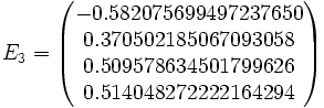
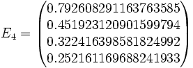
Example
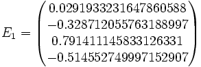
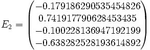
Let
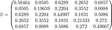
Then jacobi produces the following eigenvalues and eigenvectors after 3 sweeps (19 iterations) :


Applications for real symmetric matrices
When the eigenvalues (and eigenvectors) of a symmetric matrix are known, the following values are easily calculated.
- Singular values
- The singular values of a (square) matrix A are the square roots of the (non-negative) eigenvalues of
 . In case of a symmetric matrix S we have of
  , hence the singular values of S are the absolute values of the eigenvalues of S
- 2-norm and spectral radius
- The 2-norm of a matrix A is the norm based on the Euclidean vectornorm, i.e. the largest value
 when x runs through all vectors with
  . It is the largest singular value of A. In case of a symmetric matrix it is largest absolute value of its eigenvectors and thus equal to its spectral radius.
- Condition number
- The condition number of a nonsingular matrix A is defined as
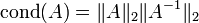 . In case of a symmetric matrix it is the absolute value of the quotient of the largest and smallest eigenvalue. Matrices with large condition numbers can cause numerically unstable results: small perturbation can result in large errors. Hilbert matrices are the most famous ill-conditioned matrices. For example, the fourth-order Hilbert matrix has a condition of 15514, while for order 8 it is 2.7 × 10⁸.
- Rank
- A matrix A has rank r if it has r columns that are linearly independent while the remaining columns are linearly dependent on these. Equivalently, r is the dimension of the range of A. Furthermore it is the number of nonzero singular values.
- In case of a symmetric matrix r is the number of nonzero eigenvalues. Unfortunately because of rounding errors numerical approximations of zero eigenvalues may not be zero (it may also happen that a numerical approximation is zero while the true value is not). Thus one can only calculate the numerical rank by making a decision which of the eigenvalues are close enough to zero.
- Pseudo-inverse
- The pseudo inverse of a matrix A is the unique matrix
 for which AX and XA are symmetric and for which AXA = A, XAX = X holds. If A is nonsingular, then '
 .
. - When procedure jacobi (S, e, E) is called, then the relation
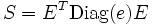 holds where Diag(e) denotes the diagonal matrix with vector e on the diagonal. Let
  denote the vector where is replaced by
  if
if  and by 0 if is (numerically close to) zero. Since matrix E is orthogonal, it follows that the pseudo-inverse of S is given by
 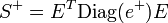 .
.
- Least squares solution
- If matrix A does not have full rank, there may not be a solution of the linear system Ax = b. However one can look for a vector x for which
 is minimal. The solution is
  . In case of a symmetric matrix S as before, one has
 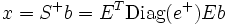 .
.
- Matrix exponential
- From one finds
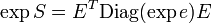 where exp e is the vector where is replaced by
  . In the same way, f(S) can be calculated in an obvious way for any (analytic) function f.
- Linear differential equations
- The differential equation x' = Ax, x(0) = a has the solution x(t) = exp(t A) a. For a symmetric matrix S, it follows that
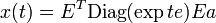 . If
. If  is the expansion of a by the eigenvectors of S, then
  .
. - Let
 be the vector space spanned by the eigenvectors of S which correspond to a negative eigenvalue and
  analogously for the positive eigenvalues. If
  then
then  i.e. the equilibrium point 0 is attractive to x(t). If
  then
then  , i.e. 0 is repulsive to x(t). and are called stable and unstable manifolds for S. If a has components in both manifolds, then one component is attracted and one component is repelled. Hence x(t) approaches as
  .
.
Generalizations
The Jacobi Method has been generalized to complex Hermitian matrices, general nonsymmetric real and complex matrices as well as block matrices.
Since singular values of a real matrix are the square roots of the eigenvalues of the symmetric matrix  it can also be used for the calculation of these values. For this case, the method is modified in such a way that S must not be explicitly calculated which reduces the danger of round-off errors. Note that
  with
with  .
.
The Jacobi Method is also well suited for parallelism.
References
- ↑ Jacobi, C.G.J. (1846). "Über ein leichtes Verfahren, die in der Theorie der Säkularstörungen vorkommenden Gleichungen numerisch aufzulösen". Crelle's Journal (in German) 30: 51–94.
- ↑ Golub, G.H.; van der Vorst, H.A. (2000). "Eigenvalue computation in the 20th century". Journal of Computational and Applied Mathematics 123 (1-2): 35–65. doi:10.1016/S0377-0427(00)00413-1.
- ↑ Schönhage, A. (1964). "Zur quadratischen Konvergenz des Jacobi-Verfahrens". Numerische Mathematik (in German) 6 (1): 410–412. doi:10.1007/BF01386091. MR 174171.
Further reading
- Press, WH; Teukolsky, SA; Vetterling, WT; Flannery, BP (2007), "Section 11.1. Jacobi Transformations of a Symmetric Matrix", Numerical Recipes: The Art of Scientific Computing (3rd ed.), New York: Cambridge University Press, ISBN 978-0-521-88068-8
- Rutishauser, H. (1966). "Handbook Series Linear Algebra: The Jacobi method for real symmetric matrices.". Numerische Mathematik 9 (1): 1–10. doi:10.1007/BF02165223. MR 1553948.
- Sameh, A.H. (1971). "On Jacobi and Jacobi-like algorithms for a parallel computer". Mathematics of Computation 25 (115): 579–590. JSTOR 2005221. MR 297131.
- Shroff, Gautam M. (1991). "A parallel algorithm for the eigenvalues and eigenvectors of a general complex matrix". Numerische Mathematik 58 (1): 779–805. doi:10.1007/BF01385654. MR 1098865.
- Veselić, K. (1979). "On a class of Jacobi-like procedures for diagonalising arbitrary real matrices". Numerische Mathematik 33 (2): 157–172. doi:10.1007/BF01399551. MR 549446.
- Veselić, K.; Wenzel, H. J. (1979). "A quadratically convergent Jacobi-like method for real matrices with complex eigenvalues". Numerische Mathematik 33 (4): 425–435. doi:10.1007/BF01399324. MR 553351.
External links
- Jacobi's Method
- Jacobi Iteration for Eigenvectors
- Matlab implementation of Jacobi algorithm that avoids trigonometric functions
| ||||||||||||||||||