Iterative proportional fitting

The iterative proportional fitting procedure (IPFP, also known as biproportional fitting in statistics, RAS algorithm^[1] in economics and matrix raking or matrix scaling in computer science) is an iterative algorithm for estimating cell values of a contingency table such that the marginal totals remain fixed and the estimated table decomposes into an outer product.

First introduced by Deming and Stephan in 1940^[2] (they proposed IPFP as an algorithm leading to a minimizer of the Pearson X-squared statistic, which it does not,^[3] and even failed to prove convergence), it has seen various extensions and related research. A rigorous proof of convergence by means of differential geometry is due to Fienberg (1970).^[4] He interpreted the family of contingency tables of constant crossproduct ratios as a particular (IJ − 1)-dimensional manifold of constant interaction and showed that the IPFP is a fixed-point iteration on that manifold. Nevertheless, he assumed strictly positive observations. Generalization to tables with zero entries is still considered a hard and only partly solved problem.

An exhaustive treatment of the algorithm and its mathematical foundations can be found in the book of Bishop et al. (1975).^[5] The first general proof of convergence, built on non-trivial measure theoretic theorems and entropy minimization, is due to Csiszár (1975).^[6] Relatively new results on convergence and error behavior have been published by Pukelsheim and Simeone (2009) .^[7] They proved simple necessary and sufficient conditions for the convergence of the IPFP for arbitrary two-way tables (i.e. tables with zero entries) by analysing an $L_1$ -error function.

Other general algorithms can be modified to yield the same limit as the IPFP, for instance the Newton–Raphson method and the EM algorithm. In most cases, IPFP is preferred due to its computational speed, numerical stability and algebraic simplicity.

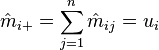
Algorithm 1 (classical IPFP)

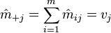
Given a two-way (I × J)-table of counts $(x_{ij})$ , where the cell values are assumed to be Poisson or multinomially distributed, we wish to estimate a decomposition $\hat{m}_{ij} = a_i b_j$ for all i and j such that $(\hat{m}_{ij})$ is the maximum likelihood estimate (MLE) of the expected values $(m_{ij})$ leaving the marginals $\textstyle x_{i+} = \sum_j x_{ij}\,$ and $\textstyle x_{+j} = \sum_i x_{ij}\,$ fixed. The assumption that the table factorizes in such a manner is known as the model of independence (I-model). Written in terms of a log-linear model, we can write this assumption as $\log\ m_{ij} = u + v_i + w_j + z_{ij}$ , where $m_{ij} := \mathbb{E}(x_{ij})$ , $\sum_i v_i = \sum_j w_j = 0$ and the interaction term vanishes, that is $z_{ij} = 0$ for all i and j.

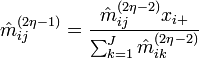
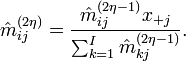
Choose initial values $\hat{m}_{ij}^{(0)} := 1$ (different choices of initial values may lead to changes in convergence behavior), and for $\eta \geq 1$ set

\hat{m}_{ij}^{(2\eta - 1)} = \frac{\hat{m}_{ij}^{(2\eta-2)}x_{i+}}{\sum_{k=1}^J \hat{m}_{ik}^{(2\eta-2)}}

\hat{m}_{ij}^{(2\eta)} = \frac{\hat{m}_{ij}^{(2\eta-1)}x_{+j}}{\sum_{k=1}^I \hat{m}_{kj}^{(2\eta-1)}}.

Notes:

Convergence does not depend on the actual distribution. Distributional assumptions are necessary for inferring that the limit 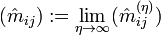$(\hat{m}_{ij}) := \lim_{\eta\rightarrow\infty} (\hat{m}^{(\eta)}_{ij})$ is an MLE indeed.

IPFP can be manipulated to generate any positive marginals be replacing $x_{i+}$ by the desired row marginal $u_i$ (analogously for the column marginals).

IPFP can be extended to fit the model of quasi-independence (Q-model), where $m_{ij} = 0$ is known a priori for $(i,j)\in S$ . Only the initial values have to be changed: Set $\hat{m}_{ij}^{(0)} = 0$ if $(i,j)\in S$ and 1 otherwise.

Algorithm 2 (factor estimation)

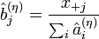
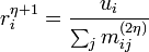
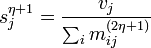
Assume the same setting as in the classical IPFP. Alternatively, we can estimate the row and column factors separately: Choose initial values $\hat{b}_j^{(0)} := 1$ , and for $\eta \geq 1$ set

\hat{a}_i^{(\eta)} = \frac{x_{i+}}{\sum_j \hat{b}_j^{(\eta-1)}},

\hat{b}_j^{(\eta)} = \frac{x_{+j}}{\sum_i \hat{a}_i^{(\eta)}}

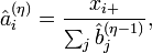
Setting 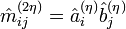$\hat{m}_{ij}^{(2\eta)} = \hat{a}_i^{(\eta)}\hat{b}_j^{(\eta)}$ , the two variants of the algorithm are mathematically equivalent (can be seen by formal induction).

Notes:

In matrix notation, we can write $(\hat{m}_{ij}) = \hat{a}\hat{b}^T$ , where $\hat{a} = (\hat{a}_1,\ldots,\hat{a}_I)^T = \lim_{\eta\rightarrow\infty} \hat{a}^{(\eta)}$ and $\hat{b} = (\hat{b}_1,\ldots,\hat{b}_J)^T = \lim_{\eta\rightarrow\infty} \hat{b}^{(\eta)}$ .
The factorization is not unique, since it is $m_{ij} = a_i b_j = (\gamma a_i)(\frac{1}{\gamma}b_j)$ for all $\gamma > 0$ .
The factor totals remain constant, i.e. $\sum_i \hat{a}_i^{(\eta)} = \sum_i \hat{a}_i^{(1)}$ for all $\eta \geq 1$ and $\sum_j \hat{b}_j^{(\eta)} = \sum_j \hat{b}_j^{(0)}$ for all $\eta \geq 0$ .
To fit the Q-model, where $m_{ij} = 0$ a priori for $(i,j)\in S$ , set $\delta_{ij} = 0$ if ( $i,j)\in S$ and $\delta_{ij} = 1$ otherwise. Then

\hat{a}_i^{(\eta)} = \frac{x_{i+}}{\sum_j \delta_{ij}\hat{b}_j^{(\eta-1)}},

\hat{b}_j^{(\eta)} = \frac{x_{+j}}{\sum_i \delta_{ij}\hat{a}_i^{(\eta)}}

\hat{m}_{ij}^{(2\eta)} = \delta_{ij}\hat{a}_i^{(\eta)}\hat{b}_j^{(\eta)}

Obviously, the I-model is a particular case of the Q-model.

Algorithm 3 (RAS)

The Problem: Let $M := (m^{(0)}_{ij}) \in \mathbb{R}^{I\times J}$ be the initial matrix with nonnegative entries, $u \in \mathbb{R}^I$ a vector of specified row marginals (e.i. row sums) and $v \in \mathbb{R}^J$ a vector of column marginals. We wish to compute a matrix $\hat{M} = (\hat{m}_{ij}) \in \mathbb{R}^{I\times J}$ similar to M and consistent with the predefined marginals, meaning

\hat{m}_{i+} = \sum_{j=1}^n \hat{m}_{ij} = u_i

and

\hat{m}_{+j} = \sum_{i=1}^m \hat{m}_{ij} = v_j

Define the diagonalization operator 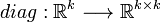$diag: \mathbb{R}^k \longrightarrow \mathbb{R}^{k\times k}$ , which produces a (diagonal) matrix with its input vector on the main diagonal and zero elsewhere. Then, for $\eta \geq 0$ , set

M^{(2\eta + 1)} = \text{diag}(r^{(\eta+1)})M^{(2\eta)}

M^{(2\eta + 2)} = M^{(2\eta+1)}\text{diag}(s^{(\eta+1)})

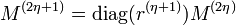
where

r_i^{\eta + 1} = \frac{u_i}{\sum_j m_{ij}^{(2\eta)}}

s_j^{\eta + 1} = \frac{v_j}{\sum_i m_{ij}^{(2\eta+1)}}

Finally, we obtain 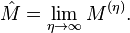$\hat{M} = \lim_{\eta\rightarrow\infty} M^{(\eta)}.$

Discussion and comparison of the algorithms

Although RAS seems to be the solution of an entirely different problem, it is indeed identical to the classical IPFP. In practice, one would not implement actual matrix multiplication, since diagonal matrices are involved. Reducing the operations to the necessary ones, it can easily be seen that RAS does the same as IPFP. The vaguely demanded 'similarity' can be explained as follows: IPFP (and thus RAS) maintains the crossproduct ratios, e.i.

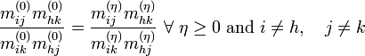
\frac{m^{(0)}_{ij}m^{(0)}_{hk}}{m^{(0)}_{ik}m^{(0)}_{hj}} = \frac{m^{(\eta)}_{ij}m^{(\eta)}_{hk}}{m^{(\eta)}_{ik}m^{(\eta)}_{hj}}\ \forall\ \eta \geq 0\text{ and }i\neq h,\quad j\neq k

since 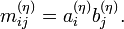$m^{(\eta)}_{ij} = a_i^{(\eta)}b_j^{(\eta)}.$

This property is sometimes called structure conservation and directly leads to the geometrical interpretation of contingency tables and the proof of convergence in the seminal paper of Fienberg (1970).

Nevertheless, direct factor estimation (algorithm 2) is under all circumstances the best way to deal with IPF: Whereas classical IPFP needs

IJ(2+J) + IJ(2+I) = I^2J + IJ^2 + 4IJ \,

elementary operations in each iteration step (including a row and a column fitting step), factor estimation needs only

I(1+J) + J(1+I) = 2IJ + I + J \,

operations being at least one order in magnitude faster than classical IPFP.

Existence and uniqueness of MLEs

Necessary and sufficient conditions for the existence and uniqueness of MLEs are complicated in the general case (see^[8]), but sufficient conditions for 2-dimensional tables are simple:

the marginals of the observed table do not vanish (that is, $x_{i+} > 0,\ x_{+j} > 0$ ) and
the observed table is inseparable (e.i. the table does not permute to a block-diagonal shape).

If unique MLEs exist, IPFP exhibits linear convergence in the worst case (Fienberg 1970), but exponential convergence has also been observed (Pukelsheim and Simeone 2009). If a direct estimator (i.e. a closed form of $(\hat{m}_{ij})$ ) exists, IPFP converges after 2 iterations. If unique MLEs do not exist, IPFP converges toward the so-called extended MLEs by design (Haberman 1974), but convergence may be arbitrarily slow and often computationally infeasible.

If all observed values are strictly positive, existence and uniqueness of MLEs and therefore convergence is ensured.

Goodness of fit

Checking if the assumption of independence is adequate, one uses the Pearson X-squared statistic

X^2 = \sum_{i,j}\frac{(x_{ij}-\hat{m_{ij}})^2}{\hat{m_{ij}}}

or alternatively the likelihood-ratio test (G-test) statistic

G = 2\sum_{i,j} x_{ij}\log\ \frac{x_{ij}}{\hat{m}_{ij}}

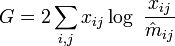Both statistics are asymptotically $\Chi^2_r$ -distributed, where $r = (I-1)(J-1)$ is the number of degrees of freedom. That is, if the p-values $1 - \Chi^2_r(X^2)$ and $1 - \Chi^2_r(G)$ are not too small (> 0.05 for instance), there is no indication to discard the hypothesis of independence.

Interpretation

If the rows correspond to different values of property A, and the columns correspond to different values of property B, and the hypothesis of independence is not discarded, the properties A and B are considered independent.

Example

Consider a table of observations (taken from the entry on contingency tables):

	right-handed	left-handed	TOTAL
male	43	9	52
female	44	4	48
TOTAL	87	13	100

For executing the classical IPFP, we first initialize the matrix with ones, leaving the marginals untouched:

	right-handed	left-handed	TOTAL
male	1	1	52
female	1	1	48
TOTAL	87	13	100

Of course, the marginal sums do not correspond to the matrix anymore, but this is fixed in the next two iterations of IPFP. The first iteration deals with the row sums:

	right-handed	left-handed	TOTAL
male	26	26	52
female	24	24	48
TOTAL	87	13	100

Note that, by definition, the row sums always constitute a perfect match after odd iterations, as do the column sums for even ones. The subsequent iteration updates the matrix column-wise:

	right-handed	left-handed	TOTAL
male	45.24	6.76	52
female	41.76	6.24	48
TOTAL	87	13	100

Now, both row and column sums of the matrix match the given marginals again.

The p-value of this matrix approximates to $p(X^2) \approx 0.1824671$ , meaning: gender and left-handedness/right-handedness can be considered independent.

Implementation

The R package mipfp (currently in version 2.0) provides a multi-dimensional implementation of the traditional iterative proportional fitting procedure.^[9] The package allows the updating a N-dimensional array with respect to given target marginal distributions (which, in turn can be multi-dimensional).

Notes

↑ Bacharach, M. (1965). "Estimating Nonnegative Matrices from Marginal Data". International Economic Review (Blackwell Publishing) 6 (3): 294–310. doi:10.2307/2525582. JSTOR 2525582.
↑ Deming, W. E.; Stephan, F. F. (1940). "On a Least Squares Adjustment of a Sampled Frequency Table When the Expected Marginal Totals are Known". Annals of Mathematical Statistics 11 (4): 427–444. doi:10.1214/aoms/1177731829. MR 3527.
↑ Stephan, F. F. (1942). "Iterative method of adjusting frequency tables when expected margins are known". Annals of Mathematical Statistics 13 (2): 166–178. doi:10.1214/aoms/1177731604. MR 6674. Zbl 0060.31505.
↑ Fienberg, S. E. (1970). "An Iterative Procedure for Estimation in Contingency Tables". Annals of Mathematical Statistics 41 (3): 907–917. doi:10.1214/aoms/1177696968. JSTOR 2239244. MR 266394. Zbl 0198.23401.
↑ Bishop, Y. M. M.; Fienberg, S. E.; Holland, P. W. (1975). Discrete Multivariate Analysis: Theory and Practice. MIT Press. ISBN 978-0-262-02113-5. MR 381130.
↑ Csiszár, I. (1975). "I-Divergence of Probability Distributions and Minimization Problems". Annals of Probability 3 (1): 146–158. doi:10.1214/aop/1176996454. JSTOR 2959270. MR 365798. Zbl 0318.60013.
↑ "On the Iterative Proportional Fitting Procedure: Structure of Accumulation Points and L1-Error Analysis". Pukelsheim, F. and Simeone, B. Retrieved 2009-06-28.
↑ Haberman, S. J. (1974). The Analysis of Frequency Data. Univ. Chicago Press. ISBN 978-0-226-31184-5.
↑ Barthélemy, Johan; Suesse, Thomas. "mipfp: Multidimensional Iterative Proportional Fitting". http://cran.r-project.org/''. CRAN. Retrieved 23 February 2015.