Invertible matrix
In linear algebra, an n-by-n square matrix A is called invertible (also nonsingular or nondegenerate) if there exists an n-by-n square matrix B such that

where In denotes the n-by-n identity matrix and the multiplication used is ordinary matrix multiplication. If this is the case, then the matrix B is uniquely determined by A and is called the inverse of A, denoted by A−1.
A square matrix that is not invertible is called singular or degenerate. A square matrix is singular if and only if its determinant is 0. Singular matrices are rare in the sense that a square matrix randomly selected from a continuous uniform distribution on its entries will almost never be singular.
Non-square matrices (m-by-n matrices for which m ≠ n) do not have an inverse. However, in some cases such a matrix may have a left inverse or right inverse. If A is m-by-n and the rank of A is equal to n, then A has a left inverse: an n-by-m matrix B such that BA = I. If A has rank m, then it has a right inverse: an n-by-m matrix B such that AB = I.
Matrix inversion is the process of finding the matrix B that satisfies the prior equation for a given invertible matrix A.
While the most common case is that of matrices over the real or complex numbers, all these definitions can be given for matrices over any commutative ring. However, in this case the condition for a square matrix to be invertible is that its determinant is invertible in the ring, which in general is a much stricter requirement than being nonzero. The conditions for existence of left-inverse resp. right-inverse are more complicated since a notion of rank does not exist over rings.
Properties
The invertible matrix theorem
Let A be a square n by n matrix over a field K (for example the field R of real numbers). The following statements are equivalent, i.e., for any given matrix they are either all true or all false:
- A is invertible, i.e. A has an inverse, is nonsingular, or is nondegenerate.
- A is row-equivalent to the n-by-n identity matrix In.
- A is column-equivalent to the n-by-n identity matrix In.
- A has n pivot positions.
- det A ≠ 0. In general, a square matrix over a commutative ring is invertible if and only if its determinant is a unit in that ring.
- A has full rank; that is, rank A = n.
- The equation Ax = 0 has only the trivial solution x = 0
- Null A = {0}
- The equation Ax = b has exactly one solution for each b in Kn.
- The columns of A are linearly independent.
- The columns of A span Kn
- Col A = Kn
- The columns of A form a basis of Kn.
- The linear transformation mapping x to Ax is a bijection from Kn to Kn.
- There is an n by n matrix B such that AB = In = BA.
- The transpose AT is an invertible matrix (hence rows of A are linearly independent, span Kn, and form a basis of Kn).
- The number 0 is not an eigenvalue of A.
- The matrix A can be expressed as a finite product of elementary matrices.
- The matrix A has a left inverse (i.e. there exists a B such that BA = I) or a right inverse (i.e. there exists a C such that AC = I), in which case both left and right inverses exist and B = C = A−1.
Other properties
Furthermore, the following properties hold for an invertible matrix A:
- (A−1)−1 = A;
- (kA)−1 = k−1A−1 for nonzero scalar k;
- (AT)−1 = (A−1)T;
- For any invertible n-by-n matrices A and B, (AB)−1 = B−1A−1. More generally, if A1,...,Ak are invertible n-by-n matrices, then (A1A2⋯Ak−1Ak)−1 = Ak−1Ak−1−1⋯A2−1A1−1;
- det(A−1) = det(A)−1.
A matrix that is its own inverse, i.e. A = A−1 and A2 = I, is called an involution.
In relation to the identity matrix
It follows from the theory of matrices that if

for finite square matrices A and B, then also

Density
Over the field of real numbers, the set of singular n-by-n matrices, considered as a subset of Rn×n, is a null set, i.e., has Lebesgue measure zero. This is true because singular matrices are the roots of the polynomial function in the entries of the matrix given by the determinant. Thus in the language of measure theory, almost all n-by-n matrices are invertible.
Furthermore the n-by-n invertible matrices are a dense open set in the topological space of all n-by-n matrices. Equivalently, the set of singular matrices is closed and nowhere dense in the space of n-by-n matrices.
In practice however, one may encounter non-invertible matrices. And in numerical calculations, matrices which are invertible, but close to a non-invertible matrix, can still be problematic; such matrices are said to be ill-conditioned.
Methods of matrix inversion
Gaussian elimination
Gauss–Jordan elimination is an algorithm that can be used to determine whether a given matrix is invertible and to find the inverse. An alternative is the LU decomposition which generates upper and lower triangular matrices which are easier to invert.
Newton's method
A generalization of Newton's method as used for a multiplicative inverse algorithm may be convenient, if it is convenient to find a suitable starting seed:

Victor Pan and John Reif have done work that includes ways of generating a starting seed.[2] [3] Byte magazine summarised one of their approaches as follows (box with equations 8 and 9 not shown):[4]-
- The Pan-Reif breakthrough consists of the discovery of a simple and reliable way of evaluating B0, the initial approximation to A−1, which can safely be used for starting Newton's iteration or variants of it. Readers interested in a derivation can consult the references. I give here merely one example of the results. Let me denote the "Hermitian transpose" of A by AH. That is, if A(I,J) is the element in the Ith row and Jth column of the A matrix, then A*(J,I) is the element at the corresponding position in the matrix A*. Here the star denotes complex conjugate (i.e., if an element is
 , where x and y are real numbers, then the complex conjugate of that element is
  ). If, as is the case to which I have limited all my own calculations, the elements of A are all real, then AH is just the transposed matrix AT of A (wherein elements are interchanged or "reflected" with respect to the main diagonal).
- We now introduce a number t, defined by equation 8. In words: We consider the magnitudes of the various elements A(I,J) of the given A matrix that is to be inverted. (In the case of a complex element , its magnitude is
 . In the case of a real element, it is just its unsigned or absolute value.) We add up the magnitudes of the elements in a given row and record the sum. We do the same for the remaining rows and then compare the sums thus obtained. The largest of these row sums - just a number - is designated
  . We do the same for the column sums and take the product of these two maxima, designating its reciprocal as the real number t. Finally, we define our initial approximate inverse matrix B0 as shown in equation 9.
- That is, the number t multiplies every element of the Hermitian transpose of the A matrix. Pan and Reif give alternative forms, but this will do. And that's all there is to it.
Otherwise, the method may be adapted to use the starting seed from a trivial starting case by using a homotopy to "walk" in small steps from that to the matrix needed, "dragging" the inverses with them:
 where
where 
 and
and  for some terminating N, perhaps followed by another few iterations at A to settle the inverse.
Using this simplistically on real valued matrices would lead the homotopy through a degenerate matrix about half the time, so complex valued matrices should be used to bypass that, e.g. by using a starting seed S that has i in the first entry, 1 on the rest of the leading diagonal, and 0 elsewhere. If complex arithmetic is not directly available, it may be emulated at a small cost in computer memory by replacing each complex matrix element a+bi with a 2×2 real valued submatrix of the form  (see square root of a matrix).
Newton's method is particularly useful when dealing with families of related matrices that behave enough like the sequence manufactured for the homotopy above: sometimes a good starting point for refining an approximation for the new inverse can be the already obtained inverse of a previous matrix that nearly matches the current matrix, e.g. the pair of sequences of inverse matrices used in obtaining matrix square roots by Denman-Beavers iteration; this may need more than one pass of the iteration at each new matrix, if they are not close enough together for just one to be enough. Newton's method is also useful for "touch up" corrections to the Gauss–Jordan algorithm which has been contaminated by small errors due to imperfect computer arithmetic.
Cayley–Hamilton method
Cayley–Hamilton theorem allows to represent the inverse of A in terms of det(A), traces and powers of A
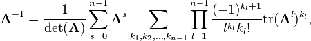
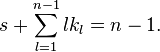
where n is dimension of A, and the sum is taken over s and the sets of all kl ≥ 0 satisfying the linear Diophantine equation
Eigen decomposition
If matrix A can be eigendecomposed and if none of its eigenvalues are zero, then A is invertible and its inverse is given by

where Q is the square (N×N) matrix whose ith column is the eigenvector  of A and Λ is the diagonal matrix whose diagonal elements are the corresponding eigenvalues, i.e.,
  .
Furthermore, because Λ is a diagonal matrix, its inverse is easy to calculate:
.
Furthermore, because Λ is a diagonal matrix, its inverse is easy to calculate:
![\left[\Lambda^{-1}\right]_{ii}=\frac{1}{\lambda_i}](../I/m/7865280dc7d7c47ac98dc6efa8975a6b.png)
Cholesky decomposition
If matrix A is positive definite, then its inverse can be obtained as
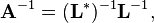
where L is the lower triangular Cholesky decomposition of A, and L* denotes the conjugate transpose of L.
Analytic solution
Writing the transpose of the matrix of cofactors, known as an adjugate matrix, can also be an efficient way to calculate the inverse of small matrices, but this recursive method is inefficient for large matrices. To determine the inverse, we calculate a matrix of cofactors:
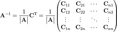
so that
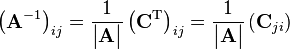
where |A| is the determinant of A, C is the matrix of cofactors, and CT represents the matrix transpose.
Inversion of 2×2 matrices
The cofactor equation listed above yields the following result for 2×2 matrices. Inversion of these matrices can be done easily as follows:[5]
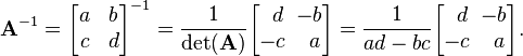
This is possible because 1/(ad-bc) is the reciprocal of the determinant of the matrix in question, and the same strategy could be used for other matrix sizes.
The Cayley–Hamilton method gives
![\mathbf{A}^{-1}=\frac{1}{\det (\mathbf{A})}\left[ \left( \mathrm{tr}\mathbf{A} \right) \mathbf{I} - \mathbf{A}\right].](../I/m/944ffd06cb2fe8b54c75a6db277a5868.png)
Inversion of 3×3 matrices
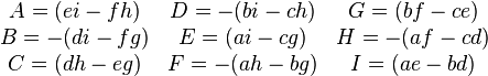
A computationally efficient 3x3 matrix inversion is given by
(where the scalar A is not to be confused with the matrix A). If the determinant is non-zero, the matrix is invertible, with the elements of the intermediary matrix on the right side above given by
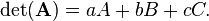
The determinant of A can be computed by applying the rule of Sarrus as follows:
The Cayley–Hamilton decomposition gives
![\mathbf{A}^{-1}=\frac{1}{\det (\mathbf{A})}\left[ \frac{1}{2}\left( (\mathrm{tr}\mathbf{A})^{2}-\mathrm{tr}\mathbf{A}^{2}\right) \mathbf{I} -\mathbf{A}\mathrm{tr}\mathbf{A}+\mathbf{A}^{2}\right].](../I/m/e00f418363ea617d2c86dcf93d3b6a63.png)
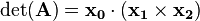
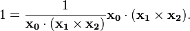
The general 3×3 inverse can be expressed concisely in terms of the cross product and triple product. If a matrix ![\mathbf{A}=\left[\mathbf{x_0},\;\mathbf{x_1},\;\mathbf{x_2}\right]](../I/m/5bea29dab57a87b59c17bbcac68a8cfc.png) (consisting of three column vectors,
(consisting of three column vectors,  ,
,  , and
, and  ) is invertible, its inverse is given by
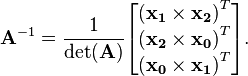
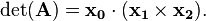
Note that  is equal to the triple product of , , and —the volume of the parallelepiped formed by the rows or columns:
The correctness of the formula can be checked by using cross- and triple-product properties and by noting that for groups, left and right inverses always coincide. Intuitively, because of the cross products, each row of  is orthogonal to the non-corresponding two columns of
  (causing the off-diagonal terms of
  be zero). Dividing by
causes the diagonal elements of to be unity. For example, the first diagonal is:
Inversion of 4×4 matrices
With increasing dimension, expressions for the inverse of A get complicated. For n = 4 the Cayley-Hamilton method leads to an expression that is still tractable:
![\mathbf{A}^{-1}=\frac{1}{\det (\mathbf{A})}\left[ \frac{1}{6}\left( (\mathrm{tr}\mathbf{A})^{3}-3\mathrm{tr}\mathbf{A}\mathrm{tr}\mathbf{A}^{2}+2\mathrm{tr}\mathbf{A}^{3}\right) \mathbf{I} -\frac{1}{2}\mathbf{A}\left( (\mathrm{tr}\mathbf{A})^{2}-\mathrm{tr}\mathbf{A}^{2}\right) +\mathbf{A}^{2}\mathrm{tr}\mathbf{A}-\mathbf{A}^{3}\right].](../I/m/1ab3c7cd6fed49d489db319b13719282.png)
Blockwise inversion
Matrices can also be inverted blockwise by using the following analytic inversion formula:
|
|
 |

where A, B, C and D are matrix sub-blocks of arbitrary size. (A and D must be square, so that they can be inverted. Furthermore, A and D−CA−1B must be nonsingular.[6]) This strategy is particularly advantageous if A is diagonal and D−CA−1B (the Schur complement of A) is a small matrix, since they are the only matrices requiring inversion. This technique was reinvented several times and is due to Hans Boltz (1923), who used it for the inversion of geodetic matrices, and Tadeusz Banachiewicz (1937), who generalized it and proved its correctness.
The nullity theorem says that the nullity of A equals the nullity of the sub-block in the lower right of the inverse matrix, and that the nullity of B equals the nullity of the sub-block in the upper right of the inverse matrix.
The inversion procedure that led to Equation (1) performed matrix block operations that operated on C and D first. Instead, if A and B are operated on first, and provided D and A−BD−1C are nonsingular ,[7] the result is
|
|
 |

Equating Equations (1) and (2) leads to
|
|
 |


where Equation (3) is the matrix inversion lemma, which is equivalent to the binomial inverse theorem.
Since a blockwise inversion of an n×n matrix requires inversion of two half-sized matrices and 6 multiplications between two half-sized matrices, it can be shown that a divide and conquer algorithm that uses blockwise inversion to invert a matrix runs with the same time complexity as the matrix multiplication algorithm that is used internally.[8] There exist matrix multiplication algorithms with a complexity of O(n2.3727) operations, while the best proven lower bound is Ω(n2 log n).[9]
By Neumann series
If a matrix A has the property that
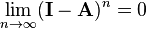
then A is nonsingular and its inverse may be expressed by a Neumann series:[10]
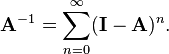
Truncating the sum results in an "approximate" inverse which may be useful as a preconditioner. Note that a truncated series can be accelerated exponentially by noting that the Neumann series is a geometric sum. Therefore, if one wishes to compute  terms, one merely need the moments
  which can be found through L matrix multiplications. Then another L matrix multiplications are needed to obtain the final result by multiplying all the moments together. Therefore, 2L matrix multiplications are needed to compute terms of the sum.
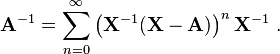
More generally, if A is "near" the invertible matrix X in the sense that

then A is nonsingular and its inverse is
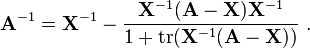
If it is also the case that A-X has rank 1 then this simplifies to
P-adic approximation
If A is an matrix with integer or rational coefficients and we seek a solution in arbitrary-precision rationals, then a p-adic approximation method converges to an exact solution in 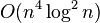 , assuming standard
  matrix multiplication is used.[11] The method relies on solving n linear systems via Dixon's method of p-adic approximation (each in
 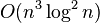 ) and is available as such in software specialized in arbitrary-precision matrix operations, e.g. in IML.[12]
Derivative of the matrix inverse
Suppose that the invertible matrix A depends on a parameter t. Then the derivative of the inverse of A with respect to t is given by
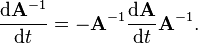
To derive the above expression for the derivative of the inverse of A, one can differentiate the definition of the matrix inverse  and then solve for the inverse of A:
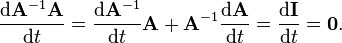
Subtracting  from both sides of the above and multiplying on the right by gives the correct expression for the derivative of the inverse:
Similarly, if  is a small number then

Moore–Penrose pseudoinverse
Some of the properties of inverse matrices are shared by Moore–Penrose pseudoinverses, which can be defined for any m-by-n matrix.
Applications
For most practical applications, it is not necessary to invert a matrix to solve a system of linear equations; however, for a unique solution, it is necessary that the matrix involved be invertible.
Decomposition techniques like LU decomposition are much faster than inversion, and various fast algorithms for special classes of linear systems have also been developed.
Regression/least squares
Although an explicit inverse is not necessary to estimate the vector of unknowns, it is unavoidable to estimate their precision, found in the diagonal of the posterior covariance matrix of the vector of unknowns.
Matrix inverses in real-time simulations
Matrix inversion plays a significant role in computer graphics, particularly in 3D graphics rendering and 3D simulations. Examples include screen-to-world ray casting, world-to-subspace-to-world object transformations, and physical simulations.
Matrix inverses in MIMO wireless communication
Matrix inversion also play a significant role in the MIMO (Multiple-Input, Multiple-Output) technology in wireless communications. The MIMO system consists of N transmit and M receive antennas. Unique signals, occupying the same frequency band, are sent via N transmit antennas and are received via M receive antennas. The signal arriving at each receive antenna will be a linear combination of the N transmitted signals forming a NxM transmission matrix H. It is crucial for the matrix H to be invertible for the receiver to be able to figure out the transmitted information.
See also
- Binomial inverse theorem
- LU decomposition
- Matrix decomposition
- Matrix square root
- Moore–Penrose pseudoinverse
- Pseudoinverse
- Singular value decomposition
- Woodbury matrix identity
Notes
- ↑ Horn, Roger A.; Johnson, Charles R. (1985). Matrix Analysis. Cambridge University Press. p. 14. ISBN 978-0-521-38632-6..
- ↑ Pan, Victor; Reif, John (1985), "Efficient Parallel Solution of Linear Systems", Proceedings of the Mth Annual ACM Symposium on Theory of Computing, Providence: ACM Missing or empty
|title=(help) - ↑ Pan, Victor; Reif, John (1985), "Harvard University Center for Research in Computing Technology Report TR-02-85", Cambridge, MA: Aiken Computation Laboratory Missing or empty
|title=(help) - ↑ "The Inversion of Large Matrices". Byte magazine 11 (04): 181–190. April 1986.
- ↑ Strang, Gilbert (2003). Introduction to linear algebra (3rd ed.). SIAM. p. 71. ISBN 0-9614088-9-8., Chapter 2, page 71
- ↑ Bernstein, Dennis (2005). Matrix Mathematics. Princeton University Press. p. 44. ISBN 0-691-11802-7.
- ↑ Bernstein, Dennis (2005). Matrix Mathematics. Princeton University Press. p. 45. ISBN 0-691-11802-7.
- ↑ T. H. Cormen, C. E. Leiserson, R. L. Rivest, C. Stein, Introduction to Algorithms, 3rd ed., MIT Press, Cambridge, MA, 2009, §28.2.
- ↑ Ran Raz. On the complexity of matrix product. In Proceedings of the thirty-fourth annual ACM symposium on Theory of computing. ACM Press, 2002. doi:10.1145/509907.509932.
- ↑ Stewart, Gilbert (1998). Matrix Algorithms: Basic decompositions. SIAM. p. 55. ISBN 0-89871-414-1.
- ↑ doi:10.1016/j.cam.2008.07.044
- ↑ https://cs.uwaterloo.ca/~astorjoh/iml.html
References
- Cormen, Thomas H.; Leiserson, Charles E., Rivest, Ronald L., Stein, Clifford (2001) [1990]. "28.4: Inverting matrices". Introduction to Algorithms (2nd ed.). MIT Press and McGraw-Hill. pp. pp. 755–760. ISBN 0-262-03293-7.
External links
- Hazewinkel, Michiel, ed. (2001), "Inversion of a matrix", Encyclopedia of Mathematics, Springer, ISBN 978-1-55608-010-4
- Matrix Mathematics: Theory, Facts, and Formulas at Google books
- Equations Solver Online
- Lecture on Inverse Matrices by Khan Academy
- Linear Algebra Lecture on Inverse Matrices by MIT
- LAPACK is a collection of FORTRAN subroutines for solving dense linear algebra problems
- ALGLIB includes a partial port of the LAPACK to C++, C#, Delphi, etc.
- Online Inverse Matrix Calculator using AJAX
- Symbolic Inverse of Matrix Calculator with steps shown
- Moore Penrose Pseudoinverse
- Inverse of a Matrix Notes
- Module for the Matrix Inverse
- Calculator for Singular or Non-Square Matrix Inverse
- The Matrix Cookbook
- Derivative of inverse matrix at PlanetMath.org.