Inverse iteration
In numerical analysis, inverse iteration is an iterative eigenvalue algorithm. It allows one to find an approximate eigenvector when an approximation to a corresponding eigenvalue is already known. The method is conceptually similar to the power method and is also known as the inverse power method. It appears to have originally been developed to compute resonance frequencies in the field of structural mechanics. [1]
The inverse power iteration algorithm starts with number  which is an approximation for the eigenvalue corresponding to the searched eigenvector,
and vector b0, which is an approximation to the eigenvector or a random vector. The method is described by the iteration
which is an approximation for the eigenvalue corresponding to the searched eigenvector,
and vector b0, which is an approximation to the eigenvector or a random vector. The method is described by the iteration
where Ck are some constants usually chosen as  Since eigenvectors are defined up to multiplication by constant, the choice of Ck can be arbitrary in theory; practical aspects of the choice of
  are discussed below.
So, at every iteration, the vector bk is multiplied by the inverse of the matrix  and normalized.
It is exactly the same formula as in the power method
modula change of matrix A, by
and normalized.
It is exactly the same formula as in the power method
modula change of matrix A, by  The better approximation to the eigenvalue is chosen, the faster convergence one gets, however incorrect choice of can lead to slow convergence or to the convergence of a different eigenvector. Usually in practice the method is used when good approximation for the eigenvalue is known, and hence one needs only few (quite often just one) iteration.
Theory and convergence
The basic idea of the power iteration is choosing an initial vector b (either an eigenvector approximation or a random vector) and iteratively calculating  . Except for a set of zero measure, for any initial vector, the result will converge to an eigenvector corresponding to the dominant eigenvalue.
The inverse iteration does the same for the matrix  , so it converges to eigenvector corresponding to the dominant eigenvalue of the matrix .
Eigenvalues of this matrix are
, so it converges to eigenvector corresponding to the dominant eigenvalue of the matrix .
Eigenvalues of this matrix are  where
where  are eigenvalues of A.
The largest of these numbers correspond to the smallest of
are eigenvalues of A.
The largest of these numbers correspond to the smallest of 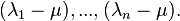 It is obvious to see that eigenvectors of matrices A and are the same. So:
Conclusion: the method converges to the eigenvector of the matrix A corresponding to the closest eigenvalue to 
In particular taking  we see that
  converges to the eigenvector corresponding the smallest in absolute value eigenvalue of A.
Speed of convergence
Let us analyze the rate of convergence of the method.
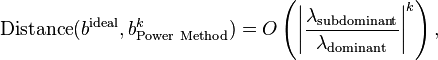
The power method is known to converge linearly to the limit, more precisely:
hence for the inverse iteration method similar result sounds as:
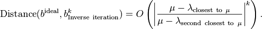
This is a key formula for understanding the method's convergence. It shows that if is chosen close enough to some eigenvalue  , for example
  each iteration will improve the accuracy
 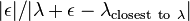 times. (We use that for small enough
  "closest to " and "closest to " is the same.) For small enough
  it is approximately the same as
 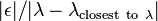 . Hence if one is able to find , such the
will be small enough, then very few iterations may be satisfactory.
. Hence if one is able to find , such the
will be small enough, then very few iterations may be satisfactory.
Complexity
The inverse iteration algorithm requires solving a linear system or calculation of the inverse matrix.
For non-structured matrices (not sparse, not Toeplitz,...) this requires  operations.
Implementation options
The method is defined by the formula:
There are several details in its implementation.
- Calculate inverse matrix or solve system of linear equations.
We can rewrite the formula in the following way:
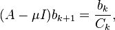
emphasizing that to find the next approximation  we need to solve a system of linear equations.
There are two options: one may choose an algorithm that solves a linear
system, or to calculate an inverse matrix
and then apply it to the vector.
Both options have complexity O(n3), the exact number depends on the chosen method. Typically, solutions of linear equations have slightly less complexity. The choice between the options depends on the number of iterations. If one solves the linear system the complexity will be k*O(n3), where k is number of iterations. Calculating the inverse matrix first and then applying it to the vectors bk is of complexity O(n3) + k* n2. The second option is clearly preferable for large numbers of iterations. As inverse iterations are typically used when only a small number of iterations is needed one usually solves a linear system of equations.
we need to solve a system of linear equations.
There are two options: one may choose an algorithm that solves a linear
system, or to calculate an inverse matrix
and then apply it to the vector.
Both options have complexity O(n3), the exact number depends on the chosen method. Typically, solutions of linear equations have slightly less complexity. The choice between the options depends on the number of iterations. If one solves the linear system the complexity will be k*O(n3), where k is number of iterations. Calculating the inverse matrix first and then applying it to the vectors bk is of complexity O(n3) + k* n2. The second option is clearly preferable for large numbers of iterations. As inverse iterations are typically used when only a small number of iterations is needed one usually solves a linear system of equations.
- Tridiagonalization, Hessenberg form.
If it is necessary to perform many iterations (or few iterations, but for many eigenvectors), then it might be wise to bring the matrix to the
upper Hessenberg form first (for symmetric matrix this will be tridiagonal form). Which costs  arithmetic operations using a technique based on Householder reduction), with a finite sequence of orthogonal similarity transforms, somewhat like a two-sided QR decomposition.[2][3] (For QR decomposition, the Householder rotations are multiplied only on the left, but for the Hessenberg case they are multiplied on both left and right.) For symmetric matrices this procedure costs
  arithmetic operations using a technique based on Householder reduction.[2][3]
Solution of the system of linear equations for the tridiagonal matrix costs O(n) operations, so the complexity grows like O(n3)+k*O(n), where k is an iteration number, which is better than for the direct inversion. However for small number of iterations such transformation may not be practical.
Also transformation to the Hessenberg form involves square roots and division operation, which are not hardware supported on some equipment like digital signal processors, FPGA, ASIC.
- Choice of the normalization constant Ck and avoiding division.
On general purpose processors (e.g. produced by Intel) the execution time of addition, multiplication and division is approximately the same. But fast and/or low energy consuming hardware (digital signal processors, FPGA , ASIC) division is not supported by hardware, and so should be avoided. For such hardware it is recommended to use Ck=2nk, since division by powers of 2 is implemented by bit shift and supported on any hardware.
The same hardware usually supports only fixed point arithmetics: essentially works with integers. So the choice of the constant Ck is especially important - taking too small value will lead to fast growth of the norm of bk and to the overflow; for too big Ck vector bk will tend to zero. The optimal value of Ck is the eigenvalue of the corresponding eigenvector. So one should choose Ck approximately the same.
Usage
The main application of the method is the situation when an approximation to an eigenvalue is found and one needs to find the corresponding approximate eigenvector. In such situation the inverse iteration is the main and probably the only method to use. So typically the method is used in combination with some other methods which allows to find approximate eigenvalues: the standard example is the bisection eigenvalue algorithm, another example is the Rayleigh quotient iteration which is actually the same inverse iteration with the choice of the approximate eigenvalue as the Rayleigh quotient corresponding to the vector obtained on the previous step of the iteration.
There are some situations where the method can be used by itself, however they are quite marginal.
Dominant eigenvector.
The dominant eigenvalue can be easily estimated for any matrix.
For any induced norm it is true that
 for any eigenvalue .
So taking the norm of the matrix as an approximate eigenvalue one can see that the method will converge to the dominant eigenvector.
for any eigenvalue .
So taking the norm of the matrix as an approximate eigenvalue one can see that the method will converge to the dominant eigenvector.
Estimates based on statistics. In some real-time applications one needs to find eigenvectors for matrices with a speed may be millions matrices per second. In such applications typically the statistics of matrices is known in advance and one can take as approximate eigenvalue the average eigenvalue for some large matrix sample, or better one calculates the mean ratio of the eigenvalue to the trace or the norm of the matrix and eigenvalue is estimated as trace or norm multiplied on the average value the their ratio. Clearly such method can be used with much care and only in situations when the mistake in calculations is allowed. Actually such idea can be combined with other methods to avoid too big errors.
See also
References
- ↑ Ernst Pohlhausen, Berechnung der Eigenschwingungen statisch-bestimmter Fachwerke, ZAMM - Zeitschrift für Angewandte Mathematik und Mechanik 1, 28-42 (1921).
- ↑ 2.0 2.1 Demmel, James W. (1997), Applied Numerical Linear Algebra, Philadelphia, PA: Society for Industrial and Applied Mathematics, ISBN 0-89871-389-7, MR 1463942.
- ↑ 3.0 3.1 Lloyd N. Trefethen and David Bau, Numerical Linear Algebra (SIAM, 1997).
External links
- Inverse Iteration to find eigenvectors, physics.arizona.edu
- The Power Method for Eigenvectors, math.fullerton.edu
| ||||||||||||||||||