Intelligent driver model

In traffic flow modeling, the intelligent driver model (IDM) is a time-continuous car-following model for the simulation of freeway and urban traffic. It was developed by Treiber, Hennecke and Helbing in 2000 to improve upon results provided with other "intelligent" driver models such as Gipps' Model, which lose realistic properties in the deterministic limit.

Model definition

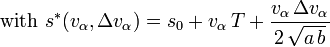
As a car-following model, the IDM describes the dynamics of the positions and velocities of single vehicles. For vehicle $\alpha$ , $x_\alpha$ denotes its position at time $t$ , and $v_\alpha$ its velocity. Furthermore, $l_\alpha$ gives the length of the vehicle. To simplify notation, we define the net distance $s_\alpha := x_{\alpha-1} - x_\alpha - l_{\alpha-1}$ , where $\alpha - 1$ refers to the vehicle directly in front of vehicle $\alpha$ , and the velocity difference, or approaching rate, 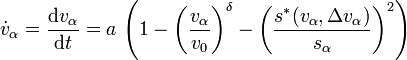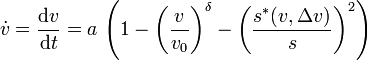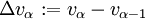$\Delta v_\alpha := v_\alpha - v_{\alpha-1}$ . For a simplified version of the model, the dynamics of vehicle $\alpha$ are then described by the following two ordinary differential equations:

\dot{x}_\alpha = \frac{\mathrm{d}x_\alpha}{\mathrm{d}t} = v_\alpha

\dot{v}_\alpha = \frac{\mathrm{d}v_\alpha}{\mathrm{d}t} = a\,\left( 1 - \left(\frac{v_\alpha}{v_0}\right)^\delta - \left(\frac{s^*(v_\alpha,\Delta v_\alpha)}{s_\alpha}\right)^2 \right)

\text{with }s^*(v_\alpha,\Delta v_\alpha) = s_0 + v_\alpha\,T + \frac{v_\alpha\,\Delta v_\alpha}{2\,\sqrt{a\,b}}

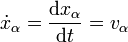
$v_0$ , $s_0$ , $T$ , $a$ , and $b$ are model parameters which have the following meaning:

desired velocity $v_0$ : the velocity the vehicle would drive at in free traffic
minimum spacing $s_0$ : a minimum desired net distance. A car can't move if the distance from the car in the front is not at least $s_0$
desired time headway $T$ : the desired time headway to the vehicle in front
acceleration $a$
comfortable braking deceleration $b$

The exponent $\delta$ is usually set to 4.

Model characteristics

The acceleration of vehicle $\alpha$ can be separated into a free road term and an interaction term:

\dot{v}^\text{free}_\alpha = a\,\left( 1 - \left(\frac{v_\alpha}{v_0}\right)^\delta \right) \qquad\dot{v}^\text{int}_\alpha = -a\,\left(\frac{s^*(v_\alpha,\Delta v_\alpha)}{s_\alpha}\right)^2 = -a\,\left(\frac{s_0 + v_\alpha\,T}{s_\alpha} + \frac{v_\alpha\,\Delta v_\alpha}{2\,\sqrt{a\,b}\,s_\alpha}\right)^2

Free road behavior: On a free road, the distance to the leading vehicle $s_\alpha$ is large and the vehicle's acceleration is dominated by the free road term, which is approximately equal to $a$ for low velocities and vanishes as $v_\alpha$ approaches $v_0$ . Therefore, a single vehicle on a free road will asymptotically approach its desired velocity $v_0$ .

Behavior at high approaching rates: For large velocity differences, the interaction term is governed by $-a\,(v_\alpha\,\Delta v_\alpha)^2\,/\,(2\,\sqrt{a\,b}\,s_\alpha)^2 = -(v_\alpha\,\Delta v_\alpha)^2\,/\,(4\,b\,s_\alpha^2)$ .

This leads to a driving behavior that compensates velocity differences while trying not to brake much harder than the comfortable braking deceleration $b$ .

Behavior at small net distances: For negligible velocity differences and small net distances, the interaction term is approximately equal to $-a\,(s_0 + v_\alpha\,T)^2\,/\,s_\alpha^2$ , which resembles a simple repulsive force such that small net distances are quickly enlarged towards an equilibrium net distance.

Solution Example

Let's assume a ring road with 50 vehicles. Then, vehicle 1 will follow vehicle 50. Initial speeds are given and since all vehicles are considered equal, vector ODEs are further simplified to:

\dot{x} = \frac{\mathrm{d}x}{\mathrm{d}t} = v

\dot{v} = \frac{\mathrm{d}v}{\mathrm{d}t} = a\,\left( 1 - \left(\frac{v}{v_0}\right)^\delta - \left(\frac{s^*(v,\Delta v)}{s}\right)^2 \right)

\text{with }s^*(v,\Delta v) = s_0 + v\,T + \frac{v\,\Delta v}{2\,\sqrt{a\,b}}

For this example, the following values are given for the equation's parameters.

Description	Value
Desired velocity	30 m/s
Safe time headway	1.5 s
Maximum acceleration	1.00 m/s²
Desired deceleration	3.00 m/s²
Acceleration exponent	4
Minimum distance	2 m
Vehicle length	5 m

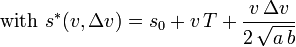
The two ordinary differential equations are solved using Runge-Kutta methods of orders 1, 3, and 5 with the same time step, to show the effects of computational accuracy in the results.

Comparison of Differential Equation Solutions for intelligent driver model using RK1,3,5

This comparison shows that the IDM does not show extremely irrealistic properties such as negative velocities or vehicles sharing the same space even for from a low order method such as with the Euler's method (RK1). However, traffic wave propagation is not as accurately represented as in the higher order methods, RK3 and RK 5. These last two methods show no significant differences, which lead to conclude that a solution for IDM reaches acceptable results from RK3 upwards and no additional computational requirements would be needed. None-the-less, when introducing heterogeneous vehicles and both jam distance parameters, this observation could not suffice.

References

Treiber, Martin; Hennecke, Ansgar; Helbing, Dirk (2000), "Congested traffic states in empirical observations and microscopic simulations", Physical Review E 62 (2): 1805–1824, doi:10.1103/PhysRevE.62.1805

Intelligent driver model

Model definition

Model characteristics

Solution Example

See also

References

External links