Indifference curve

An example of an indifference map with three indifference curves represented

In microeconomic theory, an indifference curve is a graph showing different bundles of goods between which a consumer is indifferent. That is, at each point on the curve, the consumer has no preference for one bundle over another. One can equivalently refer to each point on the indifference curve as rendering the same level of utility (satisfaction) for the consumer. In other words an indifference curve is the locus of various points showing different combinations of two goods providing equal utility to the consumer. Utility is then a device to represent preferences rather than something from which preferences come.^[1] The main use of indifference curves is in the representation of potentially observable demand patterns for individual consumers over commodity bundles.^[2]

There are infinitely many indifference curves: one passes through each combination. A collection of (selected) indifference curves, illustrated graphically, is referred to as an indifference map.

History

The theory of indifference curves was developed by Francis Ysidro Edgeworth, who explained in his book "Mathematical Psychics: an Essay on the Application of Mathematics to the Moral Sciences,” 1881,^[3] the mathematics needed for its drawing; later on, Vilfredo Pareto was the first author to actually draw these curves, in his book "Manual of Political Economy," 1906;^[4]^[5] and others in the first part of the 20th century. The theory can be derived from William Stanley Jevons's ordinal utility theory, which posits that individuals can always rank any consumption bundles by order of preference.^[6]

Map and properties of indifference curves

An example of how indifference curves are obtained as the level curves of a utility function

A graph of indifference curves for an individual consumer associated with different utility levels is called an indifference map. Points yielding different utility levels are each associated with distinct indifference curves and these indifference curves on the indifference map are like contour lines on a topographical map. Each point on the curve represents the same elevation. If you move "off" an indifference curve traveling in a northeast direction (assuming positive marginal utility for the goods) you are essentially climbing a mound of utility. The higher you go the greater the level of utility. The non-satiation requirement means that you will never reach the "top," or a "bliss point," a consumption bundle that is preferred to all others

Indifference curves are typically represented to be:

Defined only in the non-negative quadrant of commodity quantities (i.e. the possibility of having negative quantities of any good is ignored).
Negatively sloped. That is, as quantity consumed of one good (X) increases, total satisfaction would increase if not offset by a decrease in the quantity consumed of the other good (Y). Equivalently, satiation, such that more of either good (or both) is equally preferred to no increase, is excluded. (If utility U = f(x, y), U, in the third dimension, does not have a local maximum for any x and y values.) The negative slope of the indifference curve reflects the assumption of the monotonicity of consumer's preferences, which generates monotonically increasing utility functions, and the assumption of non-satiation (marginal utility for all goods is always positive); an upward sloping indifference curve would imply that a consumer is indifferent between a bundle A and another bundle B because they lie on the same indifference curve, even in the case in which the quantity of both goods in bundle B is higher. Because of monotonicity of preferences and non-satiation, a bundle with more of both goods must be preferred to one with less of both, thus the first bundle must yield a higher utility, and lie on a different indifference curve at a higher utility level. The negative slope of the indifference curve implies that the marginal rate of substitution is always positive;
Complete, such that all points on an indifference curve are ranked equally preferred and ranked either more or less preferred than every other point not on the curve. So, with (2), no two curves can intersect (otherwise non-satiation would be violated).
Transitive with respect to points on distinct indifference curves. That is, if each point on I₂ is (strictly) preferred to each point on I₁, and each point on I₃ is preferred to each point on I₂, each point on I₃ is preferred to each point on I₁. A negative slope and transitivity exclude indifference curves crossing, since straight lines from the origin on both sides of where they crossed would give opposite and intransitive preference rankings.
(Strictly) convex. With (2), convex preferences imply that the indifference curves cannot be concave to the origin, i.e. they will either be straight lines or bulge toward the origin of the indifference curve. If the latter is the case, then as a consumer decreases consumption of one good in successive units, successively larger doses of the other good are required to keep satisfaction unchanged.

Assumptions of consumer preference theory

Preferences are complete. The consumer has ranked all available alternative combinations of commodities in terms of the satisfaction they provide him.
- Assume that there are two consumption bundles A and B each containing two commodities x and y. A consumer can unambiguously determine that one and only one of the following is the case:
  - A is preferred to B ⇒ A ^p B^[7]
  - B is preferred to A ⇒ B ^p A^[7]
  - A is indifferent to B ⇒ A ^I B^[7]
    - Note that this axiom precludes the possibility that the consumer cannot decide,^[8] and that a consumer is able to make this comparison with respect to every conceivable bundle of goods.^[7]
Preferences are reflexive
- Means that if A and B are identical in all respects the consumer will recognize this fact and be indifferent in comparing A and B
  - A = B ⇒ A ^I B^[7]
Preferences are transitive^{[nb 1]}
- If A ^p B and B ^p C then A ^p C.^[7]
- Also A ^I B and B ^I C then A^I C.^[7]
  - This is a consistency assumption.
Preferences are continuous
- If A is preferred to B and C is infinitesimally close to B then A is preferred to C.
- A ^p B & C → B ⇒ A ^p C.
  - "Continuous" means infinitely divisible - just like there are infinitely many numbers between 1 and 2 all bundles are infinitely divisible. This assumption makes indifference curves continuous.
Preferences exhibit strong monotonicity
- if A has more of both x and y than B then A is preferred to B
  - this assumption is commonly called the "more is better" assumption
  - an alternative version of this assumption is strong monotonicity which requires that if A and B have the same quantity of one good, but A has more of the other, then A is preferred to B.

It also implies that the commodities are good rather than bad. Examples of bad commodities can be disease, pollution etc. because we always desire less of such things.

Indifference curves exhibit diminishing marginal rates of substitution
- The marginal rate of substitution tells how much 'y' a person is willing to sacrifice to get one more unit of 'x'.
- This assumption assures that indifference curves are smooth and convex to the origin.
- This assumption also set the stage for using techniques of constrained optimization because the shape of the curve assures that the first derivative is negative and the second is positive.
- Another name for this assumption is the substitution assumption. It is the most critical assumption of consumer theory: Consumers are willing to give up or trade-off some of one good to get more of another. The fundamental assertion is that there is a maximum amount that "a consumer will give up, of one commodity, to get one unit of another good, in that amount which will leave the consumer indifferent between the new and old situations"^[9] The negative slope of the indifference curves represents the willingness of the consumer to make a trade off.^[9]
There are also many sub-assumptions:
- Irreflexivity - for no x is x^px
- Negative transitivity - if x^not-py then for any third commodity z, either x^not-pz or z^not-py or both.

Application

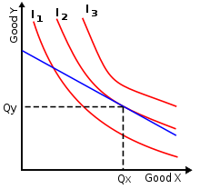
To maximise utility, a household should consume at (Qx, Qy). Assuming it does, a full demand schedule can be deduced as the price of one good fluctuates.

Consumer theory uses indifference curves and budget constraints to generate consumer demand curves. For a single consumer, this is a relatively simple process. First, let one good be an example market e.g., carrots, and let the other be a composite of all other goods. Budget constraints give a straight line on the indifference map showing all the possible distributions between the two goods; the point of maximum utility is then the point at which an indifference curve is tangent to the budget line (illustrated). This follows from common sense: if the market values a good more than the household, the household will sell it; if the market values a good less than the household, the household will buy it. The process then continues until the market's and household's marginal rates of substitution are equal.^[10] Now, if the price of carrots were to change, and the price of all other goods were to remain constant, the gradient of the budget line would also change, leading to a different point of tangency and a different quantity demanded. These price / quantity combinations can then be used to deduce a full demand curve.^[10] A line connecting all points of tangency between the indifference curve and the budget constraint is called the expansion path.^[11]

Examples of indifference curves

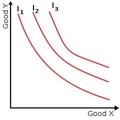
Figure 1: An example of an indifference map with three indifference curves represented
Figure 2: Three indifference curves where Goods X and Y are perfect substitutes. The gray line perpendicular to all curves indicates the curves are mutually parallel.
Figure 3: Indifference curves for perfect complements X and Y. The elbows of the curves are collinear.

In Figure 1, the consumer would rather be on I₃ than I₂, and would rather be on I₂ than I₁, but does not care where he/she is on a given indifference curve. The slope of an indifference curve (in absolute value), known by economists as the marginal rate of substitution, shows the rate at which consumers are willing to give up one good in exchange for more of the other good. For most goods the marginal rate of substitution is not constant so their indifference curves are curved. The curves are convex to the origin, describing the negative substitution effect. As price rises for a fixed money income, the consumer seeks less the expensive substitute at a lower indifference curve. The substitution effect is reinforced through the income effect of lower real income (Beattie-LaFrance). An example of a utility function that generates indifference curves of this kind is the Cobb-Douglas function $\scriptstyle U\left(x,y\right)=x^\alpha y^{1-\alpha }, 0 \leq \alpha \leq 1$ . The negative slope of the indifference curve incorporates the willingness of the consumer to make trade offs.^[9]

If two goods are perfect substitutes then the indifference curves will have a constant slope since the consumer would be willing to switch between at a fixed ratio. The marginal rate of substitution between perfect substitutes is likewise constant. An example of a utility function that is associated with indifference curves like these would be $\scriptstyle U\left(x,y\right)=\alpha x + \beta y$ .

If two goods are perfect complements then the indifference curves will be L-shaped. Examples of perfect complements include left shoes compared to right shoes: the consumer is no better off having several right shoes if she has only one left shoe - additional right shoes have zero marginal utility without more left shoes, so bundles of goods differing only in the number of right shoes they include - however many - are equally preferred. The marginal rate of substitution is either zero or infinite. An example of the type of utility function that has an indifference map like that above is the Leontief function: $\scriptstyle U\left(x,y\right)= \min \{ \alpha x, \beta y \}$ .

The different shapes of the curves imply different responses to a change in price as shown from demand analysis in consumer theory. The results will only be stated here. A price-budget-line change that kept a consumer in equilibrium on the same indifference curve:

in Fig. 1 would reduce quantity demanded of a good smoothly as price rose relatively for that good.

in Fig. 2 would have either no effect on quantity demanded of either good (at one end of the budget constraint) or would change quantity demanded from one end of the budget constraint to the other.

in Fig. 3 would have no effect on equilibrium quantities demanded, since the budget line would rotate around the corner of the indifference curve.^{[nb 2]}

Preference relations and utility

Choice theory formally represents consumers by a preference relation, and use this representation to derive indifference curves showing combinations of equal preference to the consumer.

Preference relations

Let

A\;

be a set of mutually exclusive alternatives among which a consumer can choose.

a\;

and

b\;

be generic elements of

A\;

In the language of the example above, the set $A\;$ is made of combinations of apples and bananas. The symbol $a\;$ is one such combination, such as 1 apple and 4 bananas and $b\;$ is another combination such as 2 apples and 2 bananas.

A preference relation, denoted $\succeq$ , is a binary relation define on the set $A\;$ .

The statement

a\succeq b\;

is described as ' $a\;$ is weakly preferred to $b\;$ .' That is, $a\;$ is at least as good as $b\;$ (in preference satisfaction).

The statement

a\sim b\;

is described as ' $a\;$ is weakly preferred to $b\;$ , and $b\;$ is weakly preferred to $a\;$ .' That is, one is indifferent to the choice of $a\;$ or $b\;$ , meaning not that they are unwanted but that they are equally good in satisfying preferences.

The statement

a\succ b\;

is described as ' $a\;$ is weakly preferred to $b\;$ , but $b\;$ is not weakly preferred to $a\;$ .' One says that ' $a\;$ is strictly preferred to $b\;$ .'

The preference relation $\succeq$ is complete if all pairs $a,b\;$ can be ranked. The relation is a transitive relation if whenever $a\succeq b\;$ and $b\succeq c,\;$ then $a\succeq c\;$ .

For any element $a \in A\;$ , the corresponding indifference curve, $\mathcal{C}_a$ is made up of all elements of $A\;$ which are indifferent to $a$ . Formally,

$\mathcal{C}_a=\{b \in A:b \sim a\}$ .

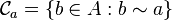Formal link to utility theory

In the example above, an element $a\;$ of the set $A\;$ is made of two numbers: The number of apples, call it $x,\;$ and the number of bananas, call it $y.\;$

In utility theory, the utility function of an agent is a function that ranks all pairs of consumption bundles by order of preference (completeness) such that any set of three or more bundles forms a transitive relation. This means that for each bundle $\left(x,y\right)$ there is a unique relation, $U\left(x,y\right)$ , representing the utility (satisfaction) relation associated with $\left(x,y\right)$ . The relation $\left(x,y\right)\to U\left(x,y\right)$ is called the utility function. The range of the function is a set of real numbers. The actual values of the function have no importance. Only the ranking of those values has content for the theory. More precisely, if $U(x,y)\geq U(x',y')$ , then the bundle $\left(x,y\right)$ is described as at least as good as the bundle $\left(x',y'\right)$ . If $U\left(x,y\right)>U\left(x',y'\right)$ , the bundle $\left(x,y\right)$ is described as strictly preferred to the bundle $\left(x',y'\right)$ .

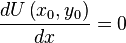
Consider a particular bundle $\left(x_0,y_0\right)$ and take the total derivative of $U\left(x,y\right)$ about this point:

dU\left(x_0,y_0\right)=U_1\left(x_0,y_0\right)dx+U_2\left(x_0,y_0\right)dy

or, without loss of generality,

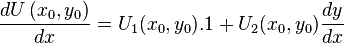\frac{dU\left(x_0,y_0\right)}{dx}= U_1(x_0,y_0).1+ U_2(x_0,y_0)\frac{dy}{dx}

(Eq. 1)

where $U_1\left(x,y\right)$ is the partial derivative of $U\left(x,y\right)$ with respect to its first argument, evaluated at $\left(x,y\right)$ . (Likewise for $U_2\left(x,y\right).$ )

The indifference curve through $\left(x_0,y_0\right)$ must deliver at each bundle on the curve the same utility level as bundle $\left(x_0,y_0\right)$ . That is, when preferences are represented by a utility function, the indifference curves are the level curves of the utility function. Therefore, if one is to change the quantity of $x\,$ by $dx\,$ , without moving off the indifference curve, one must also change the quantity of $y\,$ by an amount $dy\,$ such that, in the end, there is no change in U:

\frac{dU\left(x_0,y_0\right)}{dx}= 0

, or, substituting 0 into (Eq. 1) above to solve for dy/dx:

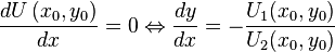\frac{dU\left(x_0,y_0\right)}{dx} = 0\Leftrightarrow\frac{dy}{dx}=-\frac{U_1(x_0,y_0)}{U_2(x_0,y_0)}

Thus, the ratio of marginal utilities gives the absolute value of the slope of the indifference curve at point $\left(x_0,y_0\right)$ . This ratio is called the marginal rate of substitution between $x\,$ and $y\,$ .

Examples

Linear utility

If the utility function is of the form $U\left(x,y\right)=\alpha x+\beta y$ then the marginal utility of $x\,$ is $U_1\left(x,y\right)=\alpha$ and the marginal utility of $y\,$ is $U_2\left(x,y\right)=\beta$ . The slope of the indifference curve is, therefore,

\frac{dx}{dy}=-\frac{\beta}{\alpha}.

Observe that the slope does not depend on $x\,$ or $y\,$ : the indifference curves are straight lines.

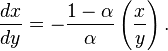
Cobb-Douglas utility

If the utility function is of the form $U\left(x,y\right)=x^\alpha y^{1-\alpha}$ the marginal utility of $x\,$ is $U_1\left(x,y\right)=\alpha \left(x/y\right)^{\alpha-1}$ and the marginal utility of $y\,$ is $U_2\left(x,y\right)=(1-\alpha) \left(x/y\right)^{\alpha}$ .Where $\alpha<1$ . The slope of the indifference curve, and therefore the negative of the marginal rate of substitution, is then

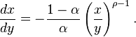
\frac{dx}{dy}=-\frac{1-\alpha}{\alpha}\left(\frac{x}{y}\right).

CES utility

A general CES (Constant Elasticity of Substitution) form is

U(x,y)=\left(\alpha x^\rho +(1-\alpha)y^\rho\right)^{1/\rho}

where $\alpha\in(0,1)$ and $\rho\leq 1$ . (The Cobb-Douglas is a special case of the CES utility, with $\rho=1\,$ .) The marginal utilities are given by

U_1(x,y)=\alpha \left(\alpha x^\rho +(1-\alpha)y^\rho\right)^{\left(1/\rho\right)-1} x^{\rho-1}

and

U_2(x,y)=(1-\alpha)\left(\alpha x^\rho +(1-\alpha)y^\rho\right)^{\left(1/\rho\right)-1} y^{\rho-1}.

Therefore, along an indifference curve,

\frac{dx}{dy}=-\frac{1-\alpha}{\alpha}\left(\frac{x}{y}\right)^{\rho-1}.

These examples might be useful for modelling individual or aggregate demand.

Biology

As used in Biology, the indifference curve is a model for how animals 'decide' whether to perform a particular behavior, based on changes in two variables which can increase in intensity, one along the x-axis and the other along the y-axis. For example, the x-axis may measure the quantity of food available while the y-axis measures the risk involved in obtaining it. The indifference curve is drawn to predict the animal's behavior at various levels of risk and food availability.

Notes

↑ The transitivity of weak preferences is sufficient for most IC analysis: If A is weakly preferred to B meaning that the consumer likes A at least as much as B and B is weakly preferred to C then A is weakly preferred to C.^[8]
↑ Indifference curves can be used to derive the individual demand curve. However, the assumptions of consumer preference theory do not guarantee that the demand curve will have a negative slope.^[12]

References

↑ Geanakoplos, John (1987). "Arrow-Debreu model of general equilibrium". The New Palgrave: A Dictionary of Economics 1. pp. 116–124 [p. 117].
↑ Böhm, Volker; Haller, Hans (1987). "Demand theory". The New Palgrave: A Dictionary of Economics 1. pp. 785–792 [p. 785].
↑ http://onlinebooks.library.upenn.edu/webbin/book/lookupid?key=olbp34052
↑ https://archive.org/details/manualedieconomi00pareuoft
↑ http://www.policonomics.com/indifference-curves/
↑ http://www.policonomics.com/william-stanley-jevons/
↑ 7.0 7.1 7.2 7.3 7.4 7.5 7.6 Binger; Hoffman (1998). Microeconomics with Calculus (2nd ed.). Reading: Addison-Wesley. pp. 109–117. ISBN 0-321-01225-9.
↑ 8.0 8.1 Perloff, Jeffrey M. (2008). Microeconomics: Theory & Applications with Calculus. Boston: Addison-Wesley. p. 62. ISBN 978-0-321-27794-7.
↑ 9.0 9.1 9.2 Silberberg; Suen (2000). The Structure of Economics: A Mathematical Analysis (3rd ed.). Boston: McGraw-Hill. ISBN 0-07-118136-9.
↑ 10.0 10.1 Lipsey, Richard G. (1975). An Introduction to Positive Economics (Fourth ed.). Weidenfeld & Nicolson. pp. 182–186. ISBN 0-297-76899-9.
↑ Salvatore, Dominick (1989). Schaum's Outline of Theory and Problems of Managerial Economics. McGraw-Hill. ISBN 0-07-054513-8.
↑ Binger; Hoffman (1998). Microeconomics with Calculus (2nd ed.). Reading: Addison-Wesley. pp. 141–143. ISBN 0-321-01225-9.

Indifference curve

History

Map and properties of indifference curves

Assumptions of consumer preference theory

Application

Examples of indifference curves

Preference relations and utility

Preference relations

Formal link to utility theory

Examples

Linear utility

Cobb-Douglas utility

CES utility

Biology

See also

Notes

References

Further reading

External links