Hyperfunction
In mathematics, hyperfunctions are generalizations of functions, as a 'jump' from one holomorphic function to another at a boundary, and can be thought of informally as distributions of infinite order. Hyperfunctions were introduced by Mikio Sato in 1958, building upon earlier work by Grothendieck and others. In Japan, they are usually called the Sato's hyperfunctions.
Formulation
A hyperfunction on the real line can be conceived of as the 'difference' between one holomorphic function defined on the upper half-plane and another on the lower half-plane. That is, a hyperfunction is specified by a pair (f, g), where f is a holomorphic function on the upper half-plane and g is a holomorphic function on the lower half-plane.
Informally, the hyperfunction is what the difference f − g would be at the real line itself. This difference is not affected by adding the same holomorphic function to both f and g, so if h is a holomorphic function on the whole complex plane, the hyperfunctions (f, g) and (f + h, g + h) are defined to be equivalent.
Definition in one dimension
The motivation can be concretely implemented using ideas from sheaf cohomology. Let  be the sheaf of holomorphic functions on C. Define the hyperfunctions on the real line by
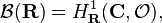
the first local cohomology group.
Concretely, let C+ and C− be the upper half-plane and lower half-plane respectively. Then
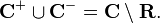
so
![H^1_{\mathbf{R}}(\mathbf{C}, \mathcal{O}) = \left [ H^0(\mathbf{C}^+, \mathcal{O}) \oplus H^0(\mathbf{C}^-, \mathcal{O}) \right ] /H^0(\mathbf{C}, \mathcal{O}).](../I/m/b719e91dae08dba88413cd02e9c88145.png)
Since the zeroth cohomology group of any sheaf is simply the global sections of that sheaf, we see that a hyperfunction is a pair of holomorphic functions one each on the upper and lower complex halfplane modulo entire holomorphic functions.
More generally one can define  for any open set
  as the quotient
 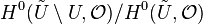 where
where  is any open set with
  . One can show that this definition does not depend on the choice of
  giving another reason to think of hyperfunctions as "boundary values" of holomorphic functions.
Examples
- If f is any holomorphic function on the whole complex plane, then the restriction of f to the real axis is a hyperfunction, represented by either (f, 0) or (0, −f).
- The Heaviside step function can be represented as
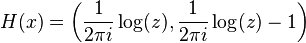 .
.
- The Dirac delta "function" is represented by
 . This is really a restatement of Cauchy's integral formula. To verify it one can calculate the integration of f just below the real line, and subtract integration of g just above the real line - both from left to right. Note that the hyperfunction can be non-trivial, even if the components are analytic continuation of the same function. Also this can be easily checked by differentiating the Heaviside function.
- If g is a continuous function (or more generally a distribution) on the real line with support contained in a bounded interval I, then g corresponds to the hyperfunction (f, −f), where f is a holomorphic function on the complement of I defined by
- This function f jumps in value by g(x) when crossing the real axis at the point x. The formula for f follows from the previous example by writing g as the convolution of itself with the Dirac delta function.
- Using a partition of unity one can write any continuous function (distribution) as a locally finite sum of functions (distributions) with compact support. This can be exploited to extend the above embedding to an embedding
 .
.
- If f is any function that is holomorphic everywhere except for an essential singularity at 0 (for example, e1/z), then (f, −f) is a hyperfunction with support 0 that is not a distribution. If f has a pole of finite order at 0 then (f, −f) is a distribution, so when f has an essential singularity then (f,−f) looks like a "distribution of infinite order" at 0. (Note that distributions always have finite order at any point.)
Operations on hyperfunctions
Let  be any open subset.
- By definition
 is a vector space such that addition and multiplication with complex numbers are well-defined. Explicitly:

- The obvious restriction maps turn
 into a sheaf (which is in fact flabby).
 - Multiplication with real analytic functions
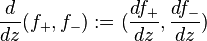
 and differentiation are well-defined:
 ,
, 
- With these definitions becomes a D-module and the embedding
 is a morphism of D-modules.
- A point
 is called a holomorphic point of
  if f restricts to a real analytic function in some small neighbourhood of a. If
  are two holomorphic points, then integration is well-defined:
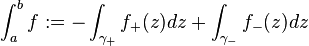
- where
![\textstyle\gamma_{\pm}:[0,1] \to \mathbb{C}^{\pm}](../I/m/aee2398285a89b1de56d96f3b4d80491.png) are arbitrary curves with
are arbitrary curves with 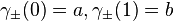 . The integrals are independent of the choice of these curves because the upper and lower half plane are simply connected.
 - Via bilinear form
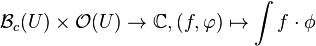 associates to each hyperfunction with compact support a continuous linear function on
  . This induces an identification of the dual space
  with the space of hyperfunctions with compact support. A special case worth considering is the case of continuous functions or distributions with compact support: If one considers
  (or
(or  ) as a subset of via the embedding from above, then this computes exactly the traditional Lebesgue-integral. Furthermore: If
  is a distribution with compact support and
  is a real analytic function, and
 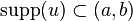 then
then 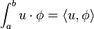 . Thus this notion of integration gives a precise meaning to formal expressions like
  which are undefined in the usual sense. Moreover: Because the real analytic functions are dense in
  , is a subspace of . This is an alternative description of the same embedding
  .
.
- If
 is a real analytic map between open sets of
  , then composition with
  is a well-defined operator
  :
:
See also
References
- Hörmander, Lars (2003), The analysis of linear partial differential operators, Volume I: Distribution theory and Fourier analysis, Berlin: Springer-Verlag, ISBN 3-540-00662-1.
- Sato, Mikio (1959), "Theory of Hyperfunctions, I", Journal of the Faculty of Science, University of Tokyo. Sect. 1, Mathematics, astronomy, physics, chemistry 8 (1): 139–193, MR 0114124, hdl:2261/6027.
- Sato, Mikio (1960), "Theory of Hyperfunctions, II", Journal of the Faculty of Science, University of Tokyo. Sect. 1, Mathematics, astronomy, physics, chemistry 8 (2): 387–437, MR 0132392, hdl:2261/6031.