Hopf bifurcation
In the mathematical theory of bifurcations, a Hopf or Poincaré–Andronov–Hopf bifurcation, named after Henri Poincaré, Eberhard Hopf, and Aleksandr Andronov, is a local bifurcation in which a fixed point of a dynamical system loses stability as a pair of complex conjugate eigenvalues of the linearization around the fixed point cross the imaginary axis of the complex plane. Under reasonably generic assumptions about the dynamical system, we can expect to see a small-amplitude limit cycle branching from the fixed point.
For a more general survey on Hopf bifurcation and dynamical systems in general, see.[1][2][3][4][5]
Overview
Supercritical / subcritical Hopf bifurcations
The limit cycle is orbitally stable if a specific quantity called the first Lyapunov coefficient is negative, and the bifurcation is supercritical. Otherwise it is unstable and the bifurcation is subcritical.
The normal form of a Hopf bifurcation is:
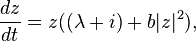
where z, b are both complex and λ is a parameter. Write

The number α is called the first Lyapunov coefficient.
- If α is negative then there is a stable limit cycle for λ > 0:
- where
- The bifurcation is then called supercritical.


- If α is positive then there is an unstable limit cycle for λ < 0. The bifurcation is called subcritical.
Remarks
The "smallest chemical reaction with Hopf bifurcation" was found in 1995 in Berlin, Germany.[6] The same biochemical system has been used in order to investigate how the existence of a Hopf bifurcation influences our ability to reverse-engineer dynamical systems.[7]
Under some general hypothesis, in the neighborhood of a Hopf bifurcation, a stable steady point of the system gives birth to a small stable limit cycle. Remark that looking for Hopf bifurcation is not equivalent to looking for stable limit cycles. First, some Hopf bifurcations (e.g. subcritical ones) do not imply the existence of stable limit cycles; second, there may exist limit cycles not related to Hopf bifurcations.
Example
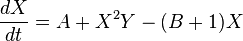
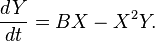
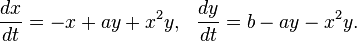
Hopf bifurcations occur in the Hodgkin–Huxley model for nerve membrane,[8] the Selkov model[9] of glycolysis, the Belousov–Zhabotinsky reaction, the Lorenz attractor and in the following simpler chemical system called the Brusselator as the parameter B changes:
The Selkov model is
The phase portrait illustrating the Hopf bifurcation in the Selkov model is shown on the right. See Strogatz, Steven H. (1994). "Nonlinear Dynamics and Chaos",[1] page 205 for detailed derivation.
Definition of a Hopf bifurcation
The appearance or the disappearance of a periodic orbit through a local change in the stability properties of a steady point is known as the Hopf bifurcation. The following theorem works with steady points with one pair of conjugate nonzero purely imaginary eigenvalues. It tells the conditions under which this bifurcation phenomenon occurs.
Theorem (see section 11.2 of [3]). Let  be the Jacobian of a continuous parametric dynamical system evaluated at a steady point
  of it. Suppose that all eigenvalues of have negative real parts except one conjugate nonzero purely imaginary pair
  . A Hopf bifurcation arises when these two eigenvalues cross the imaginary axis because of a variation of the system parameters.
Routh–Hurwitz criterion
Routh–Hurwitz criterion (section I.13 of [5]) gives necessary conditions so that a Hopf bifurcation occurs. Let us see how one can use concretely this idea.[10]
Sturm series
Let  be Sturm series associated to a characteristic polynomial
  . They can be written in the form:

The coefficients  for
for  in
in  correspond to what is called Hurwitz determinants.[10] Their definition is related to the associated Hurwitz matrix.
Propositions
Proposition 1. If all the Hurwitz determinants are positive, apart perhaps  then the associated Jacobian has no pure imaginary eigenvalues.
Proposition 2. If all Hurwitz determinants (for all in 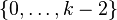 are positive,
  and
and  then all the eigenvalues of the associated Jacobian have negative real parts except a purely imaginary conjugate pair.
The conditions that we are looking for so that a Hopf bifurcation occurs (see theorem above) for a parametric continuous dynamical system are given by this last proposition.
Example
Let us consider the classical Van der Pol oscillator written with ordinary differential equations:
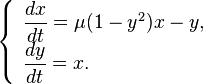
The Jacobian matrix associated to this system follows:
The characteristic polynomial (in  ) of the linearization at (0,0) is equal to:
The coefficients are:

The associated Sturm series is:
The Sturm polynomials can be written as (here  ):
):
The above proposition 2 tells that one must have:

Because 1 > 0 and −1 < 0 are obvious, one can conclude that a Hopf bifurcation may occur for Van der Pol oscillator if  .
.
See also
- Reaction–diffusion systems
References
- ↑ 1.0 1.1 Strogatz, Steven H. (1994). Nonlinear Dynamics and Chaos. Addison Wesley publishing company.
- ↑ Kuznetsov, Yuri A. (2004). Elements of Applied Bifurcation Theory. New York: Springer-Verlag. ISBN 0-387-21906-4.
- ↑ 3.0 3.1 Hale, J.; Koçak, H. (1991). Dynamics and Bifurcations. Texts in Applied Mathematics 3. New York: Springer-Verlag.
- ↑ Guckenheimer, J.; Myers, M.; Sturmfels, B. (1997). "Computing Hopf Bifurcations I". SIAM Journal on Numerical Analysis.
- ↑ 5.0 5.1 Hairer, E.; Norsett, S. P.; Wanner, G. (1993). Solving ordinary differential equations I: nonstiff problems (Second ed.). New York: Springer-Verlag.
- ↑ Wilhelm, T.; Heinrich, R. (1995). "Smallest chemical reaction system with Hopf bifurcation". Journal of Mathematical Chemistry 17 (1): 1–14. doi:10.1007/BF01165134.
- ↑ Kirk, P. D. W.; Toni, T.; Stumpf, M. P. H. (2008). "Parameter inference for biochemical systems that undergo a Hopf bifurcation". Biophysical Journal 95 (2): 540–549. doi:10.1529/biophysj.107.126086. PMC 2440454. PMID 18456830.
- ↑ Guckenheimer, J.; Labouriau, J.S. (1993), "Bifurcation of the Hodgkin and Huxley equations: A new twist", Bulletin of Mathematical Biology 55 (5): 937–952, doi:10.1007/BF02460693.
- ↑ "Selkov Model Wolfram Demo". [demonstrations.wolfram.com ]. Retrieved 30 September 2012.
- ↑ 10.0 10.1 Kahoui, M. E.; Weber, A. (2000). "Deciding Hopf bifurcations by quantifier elimination in a software component architecture". Journal of Symbolic Computation 30 (2): 161–179. doi:10.1006/jsco.1999.0353.
External links
| Wikimedia Commons has media related to Hopf bifurcations. |