Holm–Bonferroni method

In statistics, the Holm–Bonferroni method ^[1] is a method used to counteract the problem of multiple comparisons. It is intended to control the Familywise error rate and offers a simple test uniformly more powerful than the Bonferroni correction. It is one of the earliest usage of stepwise algorithms in simultaneous inference.

It is named after Sture Holm who invented the method in 1978 and Carlo Emilio Bonferroni.

Introduction

When considering several hypotheses in the same test the problem of multiplicity arises. Intuitively, the more hypotheses we check, the higher the probability to witness a rare result. With 10 different hypotheses and significance level of 0.05, the probability of committing one or more type I errors is greater than 0.4 if the nulls are in fact true. The Holm–Bonferroni method is one of many approaches that control the overall probability of witnessing one or more type I errors (aka family-wise error rate) by adjusting the rejection criteria of each of the individual hypotheses or comparisons.

Formulation

The method is as follows:

Let $H_{1},...,H_{m}$ be a family of hypotheses and $P_{1},...,P_{m}$ the corresponding P-values.
Start by ordering the p-values (from lowest to highest) $P_{(1)} \ldots P_{(m)}$ and let the associated hypotheses be $H_{(1)} \ldots H_{(m)}$
For a given significance level $\alpha$ , let $k$ be the minimal index such that $P_{(k)} > \frac{\alpha}{m+1-k}$
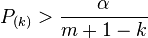
Reject the null hypotheses $H_{(1)} \ldots H_{(k-1)}$ and do not reject $H_{(k)} \ldots H_{(m)}$
If $k=1$ then do not reject any of the null hypotheses and if no such $k$ exist then reject all of the null hypotheses.

The Holm–Bonferroni method ensures that this method will control the $FWER\leq\alpha$ , where $FWER$ is the Familywise error rate

Proof that Holm-Bonferroni controls the FWER

Let $H_{(1)}\ldots H_{(m)}$ be a family of hypotheses, and $P_{(1)}\leq P_{(2)}\leq\ldots\leq P_{(m)}$ be the sorted p-values. Let $I_{0}$ be the set of indices corresponding to the (unknown) true null hypotheses, having $m_{0}$ members.

Let us assume that we wrongly reject a true hypothesis. We have to prove that the probability of this event is at most $\alpha$ . Let $h$ be the first rejected true hypothesis (first in the ordering given by the Bonferroni–Holm test). So $h-1$ is the last false hypothesis rejected and $h-1+m_0 \leq m$ . From there, we get $\frac{1}{m-h+1}\leq \frac{1}{m_0}$ (1). Since $h$ is rejected we have $P_{(h)} \leq \frac{\alpha}{m+1-h}$ by definition of the test. Using (1), the right hand side is at most $\frac{\alpha}{m_0}$ . Thus, if we wrongly reject a true hypothesis, there has to be a true hypothesis with P-value at most $\frac{\alpha}{m_0}$ .

So let us define 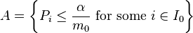$A=\left\{ P_i \leq \frac{\alpha}{m_{0}} \text{ for some } i\in I_{0}\right\}$ . Whatever the (unknown) set of true hypotheses $I_0$ is, we have $\Pr(A)\leq \alpha$ (by the Bonferroni inequalities). Therefore, the probability to reject a true hypothesis is at most $\alpha$ .

Proof that Holm-Bonferroni controls the FWER using the closure principle

The Holm–Bonferroni method can be viewed as closed testing procedure,^[2] with Bonferroni method applied locally on each of the intersections of null hypotheses.

It is a shortcut procedure since practically the number of comparisons to be made equal to $m$ or less, while the number of all intersections of null hypotheses to be tested is of order $2^m$ .

The closure principle states that a hypothesis $H_i$ in a family of hypotheses $H_1,...,H_m$ is rejected - while controlling the family-wise error rate of $\alpha$ - if and only if all the sub-families of the intersections with $H_i$ are controlled at level of family-wise error rate of $\alpha$ .

In Holm-Bonferroni procedure, we first test $H_{(1)}$ . If it is not rejected then the intersection of all null hypotheses $\bigcap\nolimits_{i = 1}^m {{H_i}}$ is not rejected too, such that there exist at least one intersection hypothesis for each of elementary hypotheses $H_1,...,H_m$ that is not rejected, thus we reject none of the elementary hypotheses.

If $H_{(1)}$ is rejected at level $\alpha/m$ then all the intersection sub-families that contain it are rejected too, thus $H_{(1)}$ is rejected. This is because $P_{(1)}$ is the smallest in each one of the intersection sub-families and the size of the sub-families is the most $m$ , such that the Bonferroni threshold larger than $\alpha/m$ .

The same rationale applies for $H_{(2)}$ . However, since $H_{(1)}$ already rejected, it sufficient to reject all the intersection sub-families of $H_{(2)}$ without $H_{(1)}$ . Once $P_{(2)}\leq\alpha/(m-1)$ holds all the intersections that contains $H_{(2)}$ are rejected.

The same applies for each $1\leq i \leq m$ .

Example

Consider four null hypotheses $H_1,...,H_4$ with unadjusted p-values $p_1=0.01$ , $p_2=0.04$ , $p_3=0.03$ and $p_4=0.005$ , to be tested at significance level $\alpha=0.05$ . Since the procedure is step-down, we first test $H_4=H_{(1)}$ , which has the smallest p-value $p_4=p_{(1)}=0.005$ . The p-value is compared to $\alpha/4=0.0125$ , the null hypothesis is rejected and we continue to the next one. Since $p_1=p_{(2)}=0.01<0.0167=\alpha/3$ we reject $H_1=H_{(2)}$ as well and continue. The next hypothesis $H_3$ is not rejected since $p_3=p_{(3)}=0.03 > 0.025=\alpha/2$ . We stop testing and conclude that $H_1$ and $H_4$ are rejected and $H_2$ and $H_3$ are not rejected while controlling the Family Wise Error Rate at level $\alpha=0.05$ . Note that even though $p_2=p_{(4)}=0.04 < 0.05=\alpha$ applies, $H_2$ is not rejected. This is because the testing procedure stops once there is no rejection.

Extensions

The Holm–Bonferroni method is an example of a closed test procedure.^[3] As such, it controls the familywise error rate for all the k hypotheses at level α in the strong sense. Each intersection is tested using the simple Bonferroni test.

Adjusted P-value

The adjusted P-values for Holm–Bonferroni method are:

\widetilde{p}_{(i)}=\max_{j\leq i}\left\{ (m-j+1)p_{(j)}\right\} _{1}

, where

\{x\}_{1}\equiv \min(x,1)

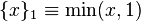In the earlier example , the adjusted p-values are $\widetilde{p}_1 = 0.03$ , $\widetilde{p}_2 = 0.06$ , $\widetilde{p}_3 = 0.06$ and $\widetilde{p}_4 = 0.02$ . Only hypotheses $H_1$ and $H_4$ are rejected at level $\alpha=0.05$ .

Šidák version

Main article: Šidák correction

When hypotheses are independent, it is possible to replace 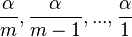$\frac{\alpha}{m},\frac{\alpha}{m-1},...,\frac{\alpha}{1}$ with:

1-(1-\alpha)^{1/m},1-(1-\alpha)^{1/(m-1)},...,1-(1-\alpha)^{1}

resulting in a slightly more powerful test.

Weighted version

Let 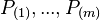$P_{(1)},...,P_{(m)}$ be the ordered unadjusted p-values. Let $H_{(i)}$ , $0\leq w_{(i)}$ correspond to $P_{(i)}$ . Reject $H_{(i)}$ as long as

P_{(j)}\leq\frac{w_{(j)}}{\sum^m_{k=j}{w_{(k)}}}\alpha,\quad j=1,...,i

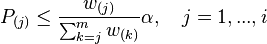
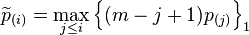
adjusted p-values: The adjusted weighted p-value are : 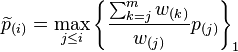$\widetilde{p}_{(i)}=\max_{j\leq i}\left\{\frac{\sum^m_{k=j}{w_{(k)}}}{w_{(j)}} p_{(j)}\right\} _{1}$ , where $\{x\}_{1}\equiv \min(x,1)$ .

A hypothesis is rejected at level α if and only if its adjusted p-value is less than α. In the earlier example using equal weights, the adjusted p-values are 0.03, 0.06, 0.06, and 0.02. This is another way to see that using α = 0.05, only hypotheses one and four are rejected by this procedure.

Alternatives and usage

Main article: Familywise error rate § Controlling procedures

Holm–Bonferroni method is uniformly more powerful than the classic Bonferroni correction. Since no assumptions required, it can always substitute the Bonferroni correction. However, it is not the best simultaneous inference controlling procedure available. There are many other methods that intend to control the family-wise error rate, many of them are more powerful than Holm-Bonferroni. Among those there is the Hochberg procedure (1988) and Hommel procedure ^[4] .

In Hochberg procedure rejection of $H_{(1)} \ldots H_{(k)}$ is made after finding the maximal index $k$ such tha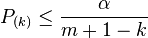t $P_{(k)} \leq \frac{\alpha}{m+1-k}$ . Thus, The Hochberg procedure is more powerful by construction. However, the Hochberg procedure require the hypotheses to be independent (or under some forms of positive dependence), while Holm-Bonferroni can be applied with no further assumptions on the data.

Bonferroni contribution

Carlo Emilio Bonferroni did not take part in inventing the method described here. Holm originally called the method the "sequentially rejective Bonferroni test", and it became known as Holm-Bonferroni only after some time. Holm's motives for naming his method after Bonferroni are explained in the original paper: "The use of the Boole inequality within multiple inference theory is usually called the Bonferroni technique, and for this reason we will call our test the sequentially rejective Bonferroni test."

References

↑ Holm, S. (1979). "A simple sequentially rejective multiple test procedure". Scandinavian Journal of Statistics 6 (2): 65–70. JSTOR 4615733. MR 538597.
↑ Marcus, R.; Peritz, E.; Gabriel, K. R. (1976). "On closed testing procedures with special reference to ordered analysis of variance". Biometrika 63 (3): 655–660. doi:10.1093/biomet/63.3.655.
↑ Marcus, R.; Peritz, E.; Gabriel, K. R. (1976). "On closed testing procedures with special reference to ordered analysis of variance". Biometrika 63 (3): 655–660. doi:10.1093/biomet/63.3.655.
↑ Hommel, G. (1988). "A stagewise rejective multiple test procedure based on a modified Bonferroni test". Biometrika 75 (2): 383–386. doi:10.1093/biomet/75.2.383. ISSN 0006-3444.