Hinge loss

Plot of hinge loss (blue) vs. zero-one loss (misclassification, green:

y < 0

) for

t = 1

and variable

y

. Note that the hinge loss penalizes predictions

y < 1

, corresponding to the notion of a margin in a support vector machine.

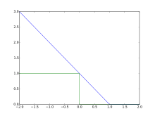
In machine learning, the hinge loss is a loss function used for training classifiers. The hinge loss is used for "maximum-margin" classification, most notably for support vector machines (SVMs).^[1] For an intended output $t = \pm1$ and a classifier score $y$ , the hinge loss of the prediction $y$ is defined as

\ell(y) = \max(0, 1-t \cdot y)

Note that $y$ should be the "raw" output of the classifier's decision function, not the predicted class label. E.g., in linear SVMs, $y = \mathbf{w} \cdot \mathbf{x} + b$ .

It can be seen that when $t$ and $y$ have the same sign (meaning $y$ predicts the right class) and $|y| \ge 1$ , the hinge loss $\ell(y) = 0$ , but when they have opposite sign, $\ell(y)$ increases linearly with $y$ (one-sided error).

Extensions

While SVMs are commonly extended to multiclass classification in a one-vs.-all or one-vs.-one fashion,^[2] there exists a "true" multiclass version of the hinge loss due to Crammer and Singer,^[3] defined for a linear classifier as^[4]

\ell(y) = \max(0, 1 + \max_{t \ne y} \mathbf{w}_t \mathbf{x} - \mathbf{w}_y \mathbf{x})

In structured prediction, the hinge loss can be further extended to structured output spaces. Structured SVMs with margin rescaling use the following variant, where $y$ denotes the SVM's parameters, $φ$ the joint feature function, and $Δ$ the Hamming loss:

\begin{align} \ell(\mathbf{y}) & = \max(0, \Delta(\mathbf{y}, \mathbf{t}) + \langle \mathbf{w}, \phi(\mathbf{x}, \mathbf{y}) \rangle - \langle \mathbf{w}, \phi(\mathbf{x}, \mathbf{t}) \rangle) \\ & = \max(0, \max_{y \in \mathcal{Y}} \left( \Delta(\mathbf{y}, \mathbf{t}) + \langle \mathbf{w}, \phi(\mathbf{x}, \mathbf{y}) \rangle \right) - \langle \mathbf{w}, \phi(\mathbf{x}, \mathbf{t}) \rangle) \end{align}

Optimization

The hinge loss is a convex function, so many of the usual convex optimizers used in machine learning can work with it. It is not differentiable, but has a subgradient with respect to model parameters $w$ of a linear SVM with score function $y = \mathbf{w} \cdot \mathbf{x}$ that is given by

\frac{\partial\ell}{\partial w_i} = \begin{cases} -t \cdot x_i & \text{if } t \cdot y < 1 \\ 0 & \text{otherwise} \end{cases}

However, since the derivative of the hinge loss at $ty = 1$ is non-deterministic, smoothed versions may be preferred for optimization, such as the quadratically smoothed

\ell(y) = \frac{1}{2\gamma} \max(0, 1 - ty)^2

suggested by Zhang.^[5] The modified Huber loss is a special case of this loss function with $\gamma = 2$ .^[5]

References

↑ Rosasco, L.; De Vito, E. D.; Caponnetto, A.; Piana, M.; Verri, A. (2004). "Are Loss Functions All the Same?". Neural Computation 16 (5): 1063–1076. doi:10.1162/089976604773135104. PMID 15070510.
↑ Duan, K. B.; Keerthi, S. S. (2005). "Which Is the Best Multiclass SVM Method? An Empirical Study". Multiple Classifier Systems. LNCS 3541. pp. 278–285. doi:10.1007/11494683_28. ISBN 978-3-540-26306-7.
↑ Crammer, Koby; Singer, Yoram (2001). "On the algorithmic implementation of multiclass kernel-based vector machines". J. Machine Learning Research 2: 265–292.
↑ Moore, Robert C.; DeNero, John (2011). "L₁ and L₂ regularization for multiclass hinge loss models". Proc. Symp. on Machine Learning in Speech and Language Processing.
↑ 5.0 5.1 Zhang, Tong (2004). Solving large scale linear prediction problems using stochastic gradient descent algorithms. ICML.