Helium atom
| Names | |
|---|---|
| Systematic IUPAC name
Helium[1] | |
| Identifiers | |
| ATC code | V03 |
| 7440-59-7 | |
| ChEBI | CHEBI:33681 |
| ChemSpider | 22423 |
| EC number | 231-168-5 |
| 16294 | |
| |
| Jmol-3D images | Image |
| KEGG | D04420 |
| MeSH | Helium |
| PubChem | 23987 |
| RTECS number | MH6520000 |
| |
| UN number | 1046 |
| Properties | |
| Molecular formula |
He |
| Molar mass | 4.00 g·mol−1 |
| Appearance | Colourless gas |
| Boiling point | −269 °C (−452.20 °F; 4.15 K) |
| Thermochemistry | |
| Std molar entropy (S |
126.151-126.155 J K−1 mol−1 |
| Hazards | |
| S-phrases | S9 |
| Except where noted otherwise, data is given for materials in their standard state (at 25 °C (77 °F), 100 kPa) | |
| | |
| Infobox references | |
- This article is about the physics of atomic helium. For other properties of helium, see helium.
A helium atom is an atom of the chemical element helium. Helium is composed of two electrons bound by the electromagnetic force to a nucleus containing two protons along with either one or two neutrons, depending on the isotope, held together by the strong force. Unlike for hydrogen, a closed-form solution to the Schrödinger equation for the helium atom has not been found. However, various approximations, such as the Hartree–Fock method, can be used to estimate the ground state energy and wavefunction of the atom.
Introduction
The Hamiltonian of helium, considered as a three-body system of two electrons and a nucleus and after separating out the centre-of-mass motion, can be written as
![H\psi(\vec{r}_1,\, \vec{r}_2) = \Bigg[\sum_{i=1,2}\Bigg(-\frac{\hbar^2}{2\mu} \nabla^2_{r_i} -\frac{Ze^2}{4\pi\epsilon_0 r_i}\Bigg) - \frac{\hbar^2}{M} \nabla_{r_1} \cdot \nabla_{r_2} + \frac{e^2}{4\pi\epsilon_0 r_{12}} \Bigg]\psi(\vec{r}_1,\, \vec{r}_2)](../I/m/0bc9aac429cc1f081d8b5c1a6dd873c2.png)
where 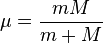 is the reduced mass of an electron with respect to the nucleus,
  and
and  are the electron-nucleus distance vectors and
 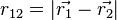 . The nuclear charge,
  is 2 for helium. In the approximation of an infinitely heavy nucleus,
  we have
  and the mass polarization term
  disappears. In atomic units the Hamiltonian simplifies to
![H\psi(\vec{r}_1,\, \vec{r}_2) = \Bigg[-\frac{1}{2}\nabla^2_{r_1} - \frac{1}{2}\nabla^2_{r_2} - \frac{Z}{r_1} - \frac{Z}{r_2} + \frac{1}{r_{12}}\Bigg]\psi(\vec{r}_1,\, \vec{r}_2).](../I/m/fc595375c99b100e8b180c34f0c65453.png)
The presence of the electron-electron interaction term 1/r12 makes this equation non separable. This means that  cannot be written as a product of one-electron wave functions and the wave function is entangled. Therefore, measurements cannot be made on one particle without affecting the other. Nevertheless, quite good theoretical descriptions of helium can be obtained within the Hartree–Fock and Thomas–Fermi approximations.
Hartree–Fock method
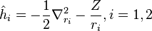
The Hartree–Fock method is used for a variety of atomic systems. However it is just an approximation, and there are more accurate and efficient methods used today to solve atomic systems. The "many-body problem" for helium and other few electron systems can be solved quite accurately. For example the ground state of helium is known to fifteen digits. In Hartree–Fock theory, the electrons are assumed to move in a potential created by the nucleus and the other electrons. The Hamiltonian for helium with two electrons can be written as a sum of the Hamiltonians for each electron:
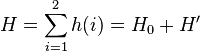
where the zero-order unperturbed Hamiltonian is
while the perturbation term:

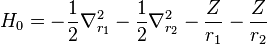
is the electron-electron interaction. H0 is just the sum of the two hydrogenic Hamiltonians:

where
En1, the energy eigenvalues and  , the corresponding eigenfunctions of the hydrogenic Hamiltonian will denote the normalized energy eigenvalues and the normalized eigenfunctions. So:

where

Neglecting the electron-electron repulsion term, the Schrödinger equation for the spatial part of the two-electron wave function will reduce to the 'zero-order' equation

This equation is separable and the eigenfunctions can be written in the form of single products of hydrogenic wave functions:

The corresponding energies are (in a.u.):
![E^{(0)}_{n_1,n_2} = E_{n_1} + E_{n_2} = - \frac{Z^2}{2} \Bigg[\frac{1}{n_1^2} + \frac{1}{n_2^2} \Bigg]](../I/m/7a4a9f609afadfba3f9ff2b6c335fd93.png)
Note that the wave function

An exchange of electron labels corresponds to the same energy  . This particular case of degeneracy with respect to exchange of electron labels is called exchange degeneracy. The exact spatial wave functions of two-electron atoms must either be symmetric or antisymmetric with respect to the interchange of the coordinates and of the two electrons. The proper wave function then must be composed of the symmetric (+) and antisymmetric(-) linear combinations:
![\psi^{(0)}_\pm(\vec{r}_1, \vec{r}_2) = \frac{1}{\sqrt{2}} [\psi_{n_1,l_1,m_1}(\vec{r}_1) \psi_{n_2,l_2,m_2}(\vec{r}_2) \pm \psi_{n_2,l_2,m_2}(\vec{r}_1) \psi_{n_1,l_1,m_1}(\vec{r}_2)]](../I/m/07d1e28267eb7a7d3cc8b7c5caa2e230.png)
This comes from Slater determinants.
The factor  normalizes
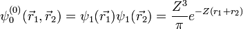
  . In order to get this wave function into a single product of one-particle wave functions, we use the fact that this is in the ground state. So
  . So the
  will vanish, in agreement with the original formulation of the Pauli exclusion principle, in which two electrons cannot be in the same state. Therefore the wave function for helium can be written as
Where  and
and  use the wave functions for the hydrogen Hamiltonian. [lower-alpha 1] For helium, Z = 2 from

where E a.u. which is approximately -108.8 eV, which corresponds to an ionization potential V
 a.u. (
 eV). The experimental values are E
 a.u. (
 eV) and V
 a.u. (
 eV).
eV).
The energy that we obtained is too low because the repulsion term between the electrons was ignored, whose effect is to raise the energy levels. As Z gets bigger, our approach should yield better results, since the electron-electron repulsion term will get smaller.
So far a very crude independent-particle approximation has been used, in which the electron-electron repulsion term is completely omitted. Splitting the Hamiltonian showed below will improve the results:

where
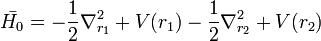
and
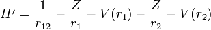
V(r) is a central potential which is chosen so that the effect of the perturbation  is small. The net effect of each electron on the motion of the other one is to screen somewhat the charge of the nucleus, so a simple guess for V(r) is

where S is a screening constant and the quantity Ze is the effective charge. The potential is a Coulomb interaction, so the corresponding individual electron energies are given (in a.u.) by

and the corresponding wave function is given by
If Ze was 1.70, that would make the expression above for the ground state energy agree with the experimental value E0 = -2.903 a.u. of the ground state energy of helium. Since Z = 2 in this case, the screening constant is S = .30. For the ground state of helium, for the average shielding approximation, the screening effect of each electron on the other one is equivalent to about  of the electronic charge.[3]
Thomas–Fermi method
Not long after Schrödinger developed the wave equation, the Thomas–Fermi model was developed. Density functional theory is used to describe the particle density  , and the ground state energy E(N), where N is the number of electrons in the atom. If there are a large number of electrons, the Schrödinger equation runs into problems, because it gets very difficult to solve, even in the atoms ground states. This is where density functional theory comes in. Thomas–Fermi theory gives very good intuition of what is happening in the ground states of atoms and molecules with N electrons.
The energy functional for an atom with N electrons is given by:

Where
The electron density needs to be greater than or equal to 0,  , and
, and  is convex.
In the energy functional, each term holds a certain meaning. The first term describes the minimum quantum-mechanical kinetic energy required to create the electron density  for an N number of electrons. The next term is the attractive interaction of the electrons with the nuclei through the Coulomb potential
  . The final term is the electron-electron repulsion potential energy.[4]
So the Hamiltonian for a system of many electrons can be written:
![H = \sum_{i=1}^N \Bigg[-\frac{\hbar^2}{2m} \nabla_i^2 + V(\vec{r_i})\Bigg] + \int \frac{e^2\rho(\vec{r'})}{|\vec{r} - \vec{r'}|} d^3r'](../I/m/3cceded85ebc3f26e58b1f1b04ca5485.png)
For helium, N = 2, so the Hamiltonian is given by:

Where
![\int \frac{e^2 \rho(\vec{r'})} {|\vec{r} - \vec{r'}|} d^3r' = \frac{e^2}{4\pi\epsilon_0} \frac{1}{|\vec{r}_1 - \vec{r}_2|},\, \text{ and }\, V(\vec{r_1}, \, \vec{r_2}) = \frac{e^2}{4\pi\epsilon_0} \Bigg[\frac{2}{r_1} + \frac{2}{r_2} \Bigg]](../I/m/849627867bb048cff2c3a95d630c3710.png)
yielding
![H = -\frac{\hbar^2}{2m} (\nabla_1^2 + \nabla_2^2) + \frac{e^2}{4\pi\epsilon_0} \Bigg[\frac{2}{r_1} + \frac{2}{r_2} - \frac{1}{|\vec{r}_1 - \vec{r}_2|}\Bigg]](../I/m/8de34b19f347ea8e555933ee8f027a3b.png)
From the Hartree–Fock method, it is known that ignoring the electron-electron repulsion term, the energy is 8E1 = -109 eV.
The variational method
To obtain a more accurate energy the variational principle can be applied to the electron-electron potential Vee using the wave function
 :
:

After integrating this, the result is:

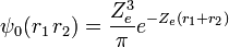
This is closer to the theoretical value, but if a better trial wave function is used, an even more accurate answer could be obtained. An ideal wave function would be one that doesn't ignore the influence of the other electron. In other words, each electron represents a cloud of negative charge which somewhat shields the nucleus so that the other electron actually sees an effective nuclear charge Z that is less than 2. A wave function of this type is given by:

Treating Z as a variational parameter to minimize H. The Hamiltonian using the wave function above is given by:

After calculating the expectation value of  and Vee the expectation value of the Hamiltonian becomes:
![\langle H \rangle = [-2Z^2 + \frac{27}{4}Z]E_1](../I/m/39ee7ffa5b66a165d38c0107e978d1c7.png)
The minimum value of Z needs to be calculated, so taking a derivative with respect to Z and setting the equation to 0 will give the minimum value of Z:
![\frac{d}{dZ} \Bigg([-2Z^2 + \frac{27}{4}Z] E_1\Bigg) = 0](../I/m/2232e9e22f72dea60b2a9cf2eb6f1e16.png)

This shows that the other electron somewhat shields the nucleus reducing the effective charge from 2 to 1.69. So we obtain the most accurate result yet:

Where again, E1 represents the ionization energy of hydrogen.
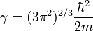
By contrast, we can also use the formula to obtain the best result:

Where  is the fine-structure constant.
By using more complicated/accurate wave functions, the ground state energy of helium has been calculated closer and closer to the experimental value -78.95 eV.[5] The variational approach has been refined to very high accuracy for a comprehensive regime of quantum states by G.W.F. Drake and co-workers[6][7][8] as well as J.D. Morgan III, Jonathan Baker and Robert Hill[9][10][11] using Hylleraas or Frankowski-Pekeris basis functions. It should be noted that one needs to include relativistic and quantum electrodynamic corrections to get full agreement with experiment to spectroscopic accuracy.[12][13]
See also
- Helium
- Hydrogen molecular ion
- Lithium atom
- Quantum mechanics
- Theoretical and experimental justification for the Schrödinger equation
- Quantum field theory
- Quantum states
- "Helium atom" on Wikiversity
- List of quantum-mechanical systems with analytical solutions
References
- ↑ For n = 1, l = 0 and m = 0, the wavefunction in a spherically symmetric potential for a hydrogen electron is
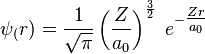 .[2] In atomic units, the Bohr radius
  equals 1, and the wavefunction becomes
 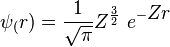 .
.
- ↑ "Helium - PubChem Public Chemical Database". The PubChem Project. USA: National Center for Biotechnology Information.
- ↑ "Hydrogen Wavefunctions". Hyperphysics. Archived from the original on 1 February 2014.
- ↑ B.H. Bransden and C.J. Joachain's Physics of Atoms and Molecules 2nd edition Pearson Education, Inc
- ↑ http://www.physics.nyu.edu/LarrySpruch/Lieb.pdf
- ↑ David I. Griffiths Introduction to Quantum Mechanics Second edition year 2005 Pearson Education, Inc
- ↑ G.W.F. Drake and Zong-Chao Van (1994). "Variational eigenvalues for the S states of helium", Chem. Phys. Lett. 229 486–490.
- ↑ Zong-Chao Yan and G. W. F. Drake (1995). "High Precision Calculation of Fine Structure Splittings in Helium and He-Like Ions", Phys. Rev. Lett. 74, 4791–4794.
- ↑ G.W.F. Drake, (1999). "High precision theory of atomic helium", Phys. Scr. T83, 83–92.
- ↑ J.D. Baker, R.N. Hill, and J.D. Morgan III (1989), "High Precision Calculation of Helium Atom Energy Levels", in AIP ConferenceProceedings 189, Relativistic, Quantum Electrodynamic, and Weak Interaction Effects in Atoms (AIP, New York),123
- ↑ Jonathan D. Baker, David E. Freund, Robert Nyden Hill, and John D. Morgan III (1990). "Radius of convergence and analytic behavior of the 1/Z expansion", Physical Review A 41, 1247.
- ↑ T.C. Scott, A. Lüchow, D. Bressanini and J.D. Morgan III (2007). The Nodal Surfaces of Helium Atom Eigenfunctions, Phys. Rev. A 75: 060101,
- ↑ G.W.F. Drake and Z.-C. Yan (1992), Phys. Rev. A 46,2378-2409. .
- ↑ G.W.F. Drake (2006). "Springer Handbook of Atomic, molecular, and Optical Physics", Edited by G.W.F. Drake (Springer, New York), 199-219.