Heaviside step function
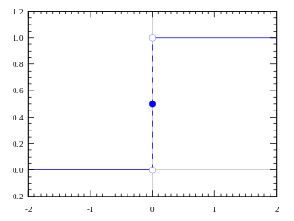
The Heaviside step function, or the unit step function, usually denoted by H (but sometimes u or θ), is a discontinuous function whose value is zero for negative argument and one for positive argument. It is an example of the general class of step functions, all of which can be represented as linear combinations of translations of this one.
It seldom matters what value is used for H(0), since H is mostly used as a distribution. Some common choices can be seen below.
The function is used in operational calculus for the solution of differential equations, and represents a signal that switches on at a specified time and stays switched on indefinitely. Oliver Heaviside, who developed the operational calculus as a method for telegraphic communications, represented the function as 1.
It is the cumulative distribution function of a random variable which is almost surely 0. (See constant random variable.)
The Heaviside function is the integral of the Dirac delta function: H′ = δ. This is sometimes written as
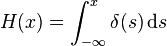
although this expansion may not hold (or even make sense) for x = 0, depending on which formalism one uses to give meaning to integrals involving δ.
Discrete form
An alternative form of the unit step, as a function of a discrete variable n:
![H[n]=\begin{cases} 0, & n < 0, \\ 1, & n \ge 0, \end{cases}](../I/m/3cc5ace7f8371cd2eaef727537ac148c.png)
where n is an integer. Unlike the usual (not discrete) case, the definition of H[0] is significant.
The discrete-time unit impulse is the first difference of the discrete-time step
![\delta\left[ n \right] = H[n] - H[n-1].](../I/m/18b1fdb556783d82836628433d71fa6d.png)
This function is the cumulative summation of the Kronecker delta:
![H[n] = \sum_{k=-\infty}^{n} \delta[k] \,](../I/m/8ac2212bc01e69e22245f783f82146fd.png)
where
![\delta[k] = \delta_{k,0} \,](../I/m/430fc704633ce64f5d7aa81d9d45df7c.png)
is the discrete unit impulse function.
Analytic approximations
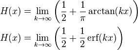
For a smooth approximation to the step function, one can use the logistic function
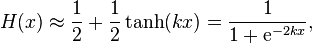
where a larger k corresponds to a sharper transition at x = 0. If we take H(0) = ½, equality holds in the limit:
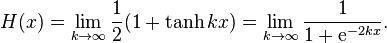
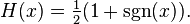
There are many other smooth, analytic approximations to the step function.[1] Among the possibilities are:
These limits hold pointwise and in the sense of distributions. In general, however, pointwise convergence need not imply distributional convergence, and vice versa distributional convergence need not imply pointwise convergence.
In general, any cumulative distribution function of a continuous probability distribution that is peaked around zero and has a parameter that controls for variance can serve as an approximation, in the limit as the variance approaches zero. For example, all three of the above approximations are cumulative distribution functions of common probability distributions: The logistic, Cauchy and normal distributions, respectively.
Integral representations
Often an integral representation of the Heaviside step function is useful:

Zero argument
Since H is usually used in integration, and the value of a function at a single point does not affect its integral, it rarely matters what particular value is chosen of H(0). Indeed when H is considered as a distribution or an element of  (see Lp space) it does not even make sense to talk of a value at zero, since such objects are only defined almost everywhere. If using some analytic approximation (as in the examples above) then often whatever happens to be the relevant limit at zero is used.
There exist various reasons for choosing a particular value.
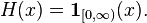
- H(0) = ½ is often used since the graph then has rotational symmetry; put another way, H-½ is then an odd function. In this case the following relation with the sign function holds for all x:
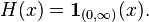
- H(0) = 1 is used when H needs to be right-continuous. For instance cumulative distribution functions are usually taken to be right continuous, as are functions integrated against in Lebesgue–Stieltjes integration. In this case H is the indicator function of a closed semi-infinite interval:
- The corresponding probability distribution is the degenerate distribution.
- H(0) = 0 is used when H needs to be left-continuous. In this case H is an indicator function of an open semi-infinite interval:
Antiderivative and derivative
The ramp function is the antiderivative of the Heaviside step function: 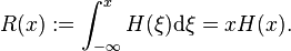
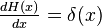
The distributional derivative of the Heaviside step function is the Dirac delta function:
Fourier transform
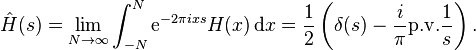
The Fourier transform of the Heaviside step function is a distribution. Using one choice of constants for the definition of the Fourier transform we have
Here  is the distribution that takes a test function
  to the Cauchy principal value of
 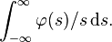 The limit appearing in the integral is also taken in the sense of (tempered) distributions.
Hyperfunction representation
This can be represented as a hyperfunction as  .
.
See also
- Rectangular function
- Step response
- Sign function
- Negative number
- Laplace transform
- Iverson bracket
- Laplacian of the indicator
- Macaulay brackets
- Sine integral
- Dirac delta function
References
- Ernst Julius Berg (1936) Heaviside's Operational Calculus, as applied to Engineering and Physics, "Unit function", page 5, McGraw-Hill Education.
- James B. Calvert (2002) Heaviside, Laplace, and the Inversion Integral, from University of Denver.
- Brian Davies (1978, 1985, 2002) Integral Transforms and their Applications, 3rd edition, page 28 "Heaviside step function", Springer.
- George F. D. Duff & D. Naylor (1966) Differential Equations of Applied Mathematics, page 42 "Heaviside unit function", John Wiley & Sons.