Harmonic map
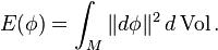
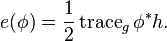
A (smooth) map φ:M→N between Riemannian manifolds M and N is called harmonic if it is a critical point of the Dirichlet energy functional
This functional E will be defined precisely below—one way of understanding it is to imagine that M is made of rubber and N made of marble (their shapes given by their respective metrics), and that the map φ:M→N prescribes how one "applies" the rubber onto the marble: E(φ) then represents the total amount of elastic potential energy resulting from tension in the rubber. In these terms, φ is a harmonic map if the rubber, when "released" but still constrained to stay everywhere in contact with the marble, already finds itself in a position of equilibrium and therefore does not "snap" into a different shape.
Harmonic maps are the 'least expanding' maps in orthogonal directions.
Existence of harmonic maps from a complete Riemannian manifold to a complete Riemannian manifold of non-positive sectional curvature was proved by Eells & Sampson (1964).
Mathematical definition
Given Riemannian manifolds (M,g), (N,h) and φ as above, the energy density of φ at a point x in M is defined as
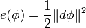
where the  is the squared norm of the differential of
  , with respect to the induced metric on the bundle
  . The total energy of φ is given by integrating the density over M
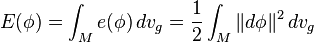
where dvg denotes the measure on M induced by its metric. This generalizes the classical Dirichlet energy.
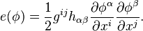
The energy density can be written more explicitly as
Using the Einstein summation convention, in local coordinates the right hand side of this equality reads
If M is compact, then φ is called a harmonic map if it is a critical point of the energy functional E. This definition is extended to the case where M is not compact by requiring the restriction of φ to every compact domain to be harmonic, or, more typically, requiring that φ be a critical point of the energy functional in the Sobolev space H1,2(M,N).
Equivalently, the map φ is harmonic if it satisfies the Euler-Lagrange equations associated to the functional E. These equations read
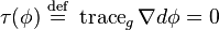
where ∇ is the connection on the vector bundle T*M⊗φ−1(TN) induced by the Levi-Civita connections on M and N. The quantity τ(φ) is a section of the bundle φ−1(TN) known as the tension field of φ. In terms of the physical analogy, it corresponds to the direction in which the "rubber" manifold M will tend to move in N in seeking the energy-minimizing configuration.
Examples
- Identity and constant maps are harmonic.
- Assume that the source manifold M is the real line R (or the circle S1), i.e. that φ is a curve (or a closed curve) on N. Then φ is a harmonic map if and only if it is a geodesic. (In this case, the rubber-and-marble analogy described above reduces to the usual elastic band analogy for geodesics.)
- Assume that the target manifold N is Euclidean space Rn (with its standard metric). Then φ is a harmonic map if and only if it is a harmonic function in the usual sense (i.e. a solution of the Laplace equation). This follows from the Dirichlet principle. If φ is a diffeomorphism onto an open set in Rn, then it gives a harmonic coordinate system.
- Every minimal surface in Euclidean space is a harmonic immersion.
- More generally, a minimal submanifold M of N is a harmonic immersion of M in N.
- Every totally geodesic map is harmonic (in this case, ∇dφ*h itself vanishes, not just its trace).
- Every holomorphic map between Kähler manifolds is harmonic.
- Every harmonic morphism between Riemannian manifolds is harmonic.
Problems and applications
- If, after applying the rubber M onto the marble N via some map φ, one "releases" it, it will try to "snap" into a position of least tension. This "physical" observation leads to the following mathematical problem: given a homotopy class of maps from M to N, does it contain a representative that is a harmonic map?
- Existence results on harmonic maps between manifolds has consequences for their curvature.
- Once existence is known, how can a harmonic map be constructed explicitly? (One fruitful method uses twistor theory.)
- In theoretical physics, a quantum field theory whose action is given by the Dirichlet energy is known as a sigma model. In such a theory, harmonic maps correspond to instantons.
- One of the original ideas in grid generation methods for computational fluid dynamics and computational physics was to use either conformal or harmonic mapping to generate regular grids.
Harmonic maps between metric spaces
The energy integral can be formulated in a weaker setting for functions u : M → N between two metric spaces (Jost 1995). The energy integrand is instead a function of the form
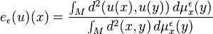
in which με
x is a family of measures attached to each point of M.
References
- Eells, J.; Sampson, J.H. (1964), "Harmonic mappings of Riemannian manifolds", Amer. J. Math. 86: 109–160, JSTOR 2373037.
- Eells, J.; Lemaire, J. (1978), "A report on harmonic maps", Bull. London Math. Soc. 10: 1–68, doi:10.1112/blms/10.1.1.
- Eells, J.; Lemaire, J. (1988), "Another report on harmonic maps", Bull. London Math. Soc. 20: 385–524, doi:10.1112/blms/20.5.385.
- Jost, Jürgen (1994), "Equilibrium maps between metric spaces", Calculus of Variations and Partial Differential Equations 2 (2): 173–204, doi:10.1007/BF01191341, ISSN 0944-2669, MR 1385525.
- Jost, Jürgen (2005), Riemannian Geometry and Geometric Analysis (4th ed.), Berlin, New York: Springer-Verlag, ISBN 978-3-540-25907-7.