Hamiltonian (control theory)
The Hamiltonian of optimal control theory was developed by Lev Pontryagin as part of his minimum principle.[1] It was inspired by, but is distinct from, the Hamiltonian of classical mechanics. Pontryagin proved that a necessary condition for solving the optimal control problem is that the control should be chosen so as to minimize the Hamiltonian. For details see Pontryagin's minimum principle.
Notation and Problem statement
A control  is to be chosen so as to minimize the objective function
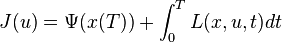
where  is the system state, which evolves according to the state equations
![\dot{x}=f(x,u,t) \qquad x(0)=x_0 \quad t \in [0,T]](../I/m/da94a0c2c4d41239da1a75f860378e99.png)
and the control must satisfy the constraints
![a \le u(t) \le b \quad t \in [0,T]](../I/m/effbb88d89d5bd9964309d744a3faf54.png)
Definition of the Hamiltonian

where  is a vector of costate variables of the same dimension as the state variables .
For information on the properties of the Hamiltonian, see Pontryagin's minimum principle.
The Hamiltonian in discrete time
When the problem is formulated in discrete time, the Hamiltonian is defined as:

and the costate equations are
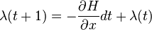
(Note that the discrete time Hamiltonian at time  involves the costate variable at time
  [2] This small detail is essential so that when we differentiate with respect to
  we get a term involving
  on the right hand side of the costate equations. Using a wrong convention here can lead to incorrect results, i.e. a costate equation which is not a backwards difference equation).
The Hamiltonian of control compared to the Hamiltonian of mechanics
William Rowan Hamilton defined the Hamiltonian as a function of three variables:

where  is defined implicitly by

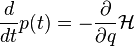
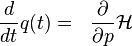
Hamilton then formulated his equations as
In contrast the Hamiltonian of control theory (as defined by Pontryagin) is a function of 4 variables

and the associated conditions for a maximum are


This difference is somewhat confusing, nevertheless a specific problem, such as the Brachystochrone problem, can be solved by either method. For details, see the article by Sussmann and Willems.[3]
References
- ↑ I. M. Ross A Primer on Pontryagin's Principle in Optimal Control, Collegiate Publishers, 2009.
- ↑ Varaiya, Chapter 6
- ↑ Sussmann; Willems (June 1997). "300 Years of Optimal Control". IEEE Control Systems.
External links
- P. Varaiya: Lecture Notes on Optimization, 2d. ed. (1998)
- I. M. Ross, Pontryagin's Hamiltonian Illustrated with Examples, 2009, Chapter 2 download