Girsanov theorem

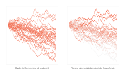
Visualisation of the Girsanov theorem — The left side shows a Wiener process with negative drift under a canonical measure P; on the right side each path of the process is colored according to its likelihood under the martingale measure Q. The density transformation from P to Q is given by the Girsanov theorem.

In probability theory, the Girsanov theorem (named after Igor Vladimirovich Girsanov) describes how the dynamics of stochastic processes change when the original measure is changed to an equivalent probability measure.^[1]^:607 The theorem is especially important in the theory of financial mathematics as it tells how to convert from the physical measure which describes the probability that an underlying instrument (such as a share price or interest rate) will take a particular value or values to the risk-neutral measure which is a very useful tool for pricing derivatives on the underlying.

History

Results of this type were first proved by Cameron–Martin in the 1940s and by Girsanov in 1960. They have been subsequently extended to more general classes of process culminating in the general form of Lenglart (1977).

Significance

Girsanov's theorem is important in the general theory of stochastic processes since it enables the key result that if Q is a measure absolutely continuous with respect to P then every P-semimartingale is a Q-semimartingale.

Statement of theorem

We state the theorem first for the special case when the underlying stochastic process is a Wiener process. This special case is sufficient for risk-neutral pricing in the Black-Scholes model and in many other models (e.g. all continuous models).

Let $\{W_t\}$ be a Wiener process on the Wiener probability space $\{\Omega,\mathcal{F},P\}$ . Let $X_t$ be a measurable process adapted to the natural filtration of the Wiener process $\{\mathcal{F}^W_t\}$ .

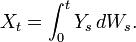
Given an adapted process $X_t$ with $X_0 = 0$ define

Z_t=\mathcal{E} (X)_t,\,

where $\mathcal{E}(X)$ is the stochastic exponential (or Doléans exponential) of X with respect to W, i.e.

\mathcal{E}(X)_t=\exp \left ( X_t - \frac{1}{2} [X]_t \right ),

where $[X]_t$ is a quadratic variation for $X_t$ . If $Z_t$ is a strictly positive martingale, a probability measure Q can be defined on $\{\Omega,\mathcal{F}\}$ such that we have Radon–Nikodym derivative

\frac{d Q}{d P} |_{\mathcal{F}_t} = Z_t = \mathcal{E} (X )_t

Then for each t the measure Q restricted to the unaugmented sigma fields $\mathcal{F}^W_t$ is equivalent to P restricted to $\mathcal{F}^W_t.\,$

Furthermore if Y is a local martingale under P then the process

\tilde Y_t = Y_t - \left[ Y,X \right]_t

is a Q local martingale on the filtered probability space $\{\Omega,F,Q,\{F^W_t\}\}$ .

Corollary

If X is a continuous process and W is Brownian motion under measure P then

\tilde W_t =W_t - \left [ W, X \right]_t

is Brownian motion under Q.

The fact that $\tilde W_t$ is continuous is trivial; by Girsanov's theorem it is a Q local martingale, and by computing the quadratic variation

\left[\tilde W \right]_t= \left[W_t, W_t\right] - 2 \left[W_t, [W, X]_t\right] + \left[[W, X]_t, [W, X]_t \right] = \left [ W \right]_t = t

it follows by Lévy's characterization of Brownian motion that this is a Q Brownian motion.

Comments

In many common applications, the process X is defined by

X_t = \int_0^t Y_s\, d W_s.

For X of this form then a sufficient condition for $\mathcal{E}(X)$ to be a martingale is Novikov's condition which requires that

E_P\left [\exp\left (\frac{1}{2}\int_0^T Y_s^2\, ds\right )\right ] < \infty.

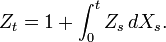
The stochastic exponential $\mathcal{E}(X)$ is the process Z which solves the stochastic differential equation

Z_t = 1 + \int_0^t Z_s\, d X_s.\,

The measure Q constructed above is not equivalent to P on $\mathcal{F}_\infty$ as this would only be the case if the Radon–Nikodym derivative were a uniformly integrable martingale, which the exponential martingale described above is not (for $\lambda\ne0$ ).

Application to finance

In finance, Girsanov theorem is used each time one needs to derive an asset's or rate's dynamics under a new probability measure. The most well known case is moving from historic measure P to risk neutral measure Q which is done - in Black Scholes framework - via Radon–Nikodym derivative:

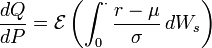
$\frac{d Q}{d P} = \mathcal{E}\left ( \int_0^\cdot \frac{r - \mu }{\sigma}\, d W_s \right )$

where $r$ denotes the instantaneous risk free rate, $\mu$ the asset's drift and $\sigma$ its volatility.

Other classical applications of Girsanov theorem are quanto adjustments and the calculation of forwards' drifts under LIBOR market model.

References

C. Dellacherie and P.-A. Meyer, "Probabilités et potentiel -- Théorie de Martingales" Chapitre VII, Hermann 1980
Girsanov, I. V., "On transforming a certain class of stochastic processes by absolutely continuous substitution of measures", Theory of Probability and its Applications, 1960
E. Lenglart "Transformation de martingales locales par changement absolue continu de probabilités", Zeitschrift für Wahrscheinlichkeit 39 (1977) pp 65–70.

External links

↑ M. Musiela, M. Rutkowski: Martingale methods in financial modelling. 2nd ed. New York : Springer-Verlag, 2004. Print.

Notes on Stochastic Calculus which contains a simple outline proof of Girsanov's theorem.
Applied Multidimensional Girsanov Theorem which contains financial applications of Girsanov's theorem.