Generalized inverse Gaussian distribution
|
Probability density function
| |
| Parameters | a > 0, b > 0, p real |
|---|---|
| Support | x > 0 |
 | |
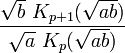
| Mean |
 |
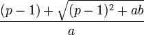
| Mode |
 |
| Variance |
![\left(\frac{b}{a}\right)\left[\frac{K_{p+2}(\sqrt{ab})}{K_p(\sqrt{ab})}-\left(\frac{K_{p+1}(\sqrt{ab})}{K_p(\sqrt{ab})}\right)^2\right]](../I/m/1731dfd5cec681cbb78eb499a7c9c358.png) |
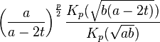
| MGF |
 |
| CF |
 |
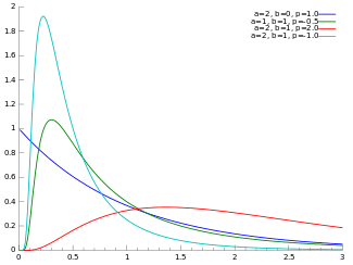
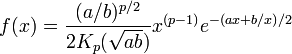
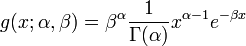
In probability theory and statistics, the generalized inverse Gaussian distribution (GIG) is a three-parameter family of continuous probability distributions with probability density function
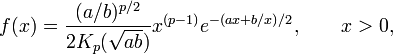
where Kp is a modified Bessel function of the second kind, a > 0, b > 0 and p a real parameter. It is used extensively in geostatistics, statistical linguistics, finance, etc. This distribution was first proposed by Étienne Halphen.[1][2][3] It was rediscovered and popularised by Ole Barndorff-Nielsen, who called it the generalized inverse Gaussian distribution. It is also known as the Sichel distribution, after Herbert Sichel.[4] Its statistical properties are discussed in Bent Jørgensen's lecture notes.[5]
Properties
Summation
Barndorff-Nielsen and Halgreen proved that the GIG distribution has Infinite divisibility[6]
Entropy
The entropy of the generalized inverse Gaussian distribution is given as
![H(f(x))=\frac{1}{2} \log \left(\frac{b}{a}\right)+\log \left(2 K_p\left(\sqrt{a b}\right)\right)-
(p-1) \frac{\left[\frac{d}{d\nu}K_\nu\left(\sqrt{ab}\right)\right]_{\nu=p}}{K_p\left(\sqrt{a b}\right)}+\frac{\sqrt{a b}}{2 K_p\left(\sqrt{a b}\right)}\left( K_{p+1}\left(\sqrt{a b}\right) + K_{p-1}\left(\sqrt{a b}\right)\right)](../I/m/e0e880a1a9828da648dd19ba87014578.png)
where ![\left[\frac{d}{d\nu}K_\nu\left(\sqrt{a b}\right)\right]_{\nu=p}](../I/m/b945f4e904eb1e6d38f1bd7850589a29.png) is a derivative of the modified Bessel function of the second kind with respect to the order
is a derivative of the modified Bessel function of the second kind with respect to the order  evaluated at
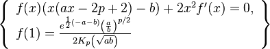
Differential equation
The pdf of the generalized inverse Gaussian distribution is a solution to the following differential equation:
Related distributions
Special cases
The inverse Gaussian and gamma distributions are special cases of the generalized inverse Gaussian distribution for p = -1/2 and b = 0, respectively.[7] Specifically, an inverse Gaussian distribution of the form
![f(x;\mu,\lambda) = \left[\frac{\lambda}{2 \pi x^3}\right]^{1/2} \exp{\frac{-\lambda (x-\mu)^2}{2 \mu^2 x}}](../I/m/14b32d96e7fcbbd2b08cab10865aa654.png)
is a GIG with  ,
,  , and
, and  . A Gamma distribution of the form
is a GIG with  ,
,  , and
, and  .
.
Other special cases include the inverse-gamma distribution, for a=0, and the hyperbolic distribution, for p=0.[7]
Conjugate prior for Gaussian
The GIG distribution is conjugate to the normal distribution when serving as the mixing distribution in a normal variance-mean mixture.[8][9] Let the prior distribution for some hidden variable, say  , be GIG:

and let there be  observed data points,
  , with normal likelihood function, conditioned on :
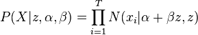
where  is the normal distribution, with mean
  and variance
  . Then the posterior for , given the data is also GIG:

where  .[note 1]
Notes
- ↑ Due to the conjugacy, these details can be derived without solving integrals, by noting that
 .
.
, the right-hand-side can be simplified to give an un-normalized GIG distribution, from which the posterior parameters can be identified.
References
- ↑ Seshadri, V. (1997). "Halphen's laws". In Kotz, S.; Read, C. B.; Banks, D. L. Encyclopedia of Statistical Sciences, Update Volume 1. New York: Wiley. pp. 302–306.
- ↑ Perreault, L.; Bobée, B.; Rasmussen, P. F. (1999). "Halphen Distribution System. I: Mathematical and Statistical Properties". Journal of Hydrologic Engineering 4 (3): 189. doi:10.1061/(ASCE)1084-0699(1999)4:3(189).
- ↑ Étienne Halphen was the uncle of the mathematician Georges Henri Halphen.
- ↑ Sichel, H.S., Statistical valuation of diamondiferous deposits, Journal of the South African Institute of Mining and Metallurgy 1973
- ↑ Jørgensen, Bent (1982). Statistical Properties of the Generalized Inverse Gaussian Distribution. Lecture Notes in Statistics 9. New York–Berlin: Springer-Verlag. ISBN 0-387-90665-7. MR 0648107.
- ↑ O. Barndorff-Nielsen and Christian Halgreen, Infinite Divisibility of the Hyperbolic and Generalized Inverse Gaussian Distributions, Zeitschrift für Wahrscheinlichkeitstheorie und verwandte Gebiete 1977
- ↑ 7.0 7.1 Johnson, Norman L.; Kotz, Samuel; Balakrishnan, N. (1994), Continuous univariate distributions. Vol. 1, Wiley Series in Probability and Mathematical Statistics: Applied Probability and Statistics (2nd ed.), New York: John Wiley & Sons, pp. 284–285, ISBN 978-0-471-58495-7, MR 1299979
- ↑ Dimitris Karlis, "An EM type algorithm for maximum likelihood estimation of the normal–inverse Gaussian distribution", Statistics & Probability Letters 57 (2002) 43–52.
- ↑ Barndorf-Nielsen, O.E., 1997. Normal Inverse Gaussian Distributions and stochastic volatility modelling. Scand. J. Statist. 24, 1–13.