General Circulation Model

Climate models are systems of differential equations based on the basic laws of physics, fluid motion, and chemistry. To “run” a model, scientists divide the planet into a 3-dimensional grid, apply the basic equations, and evaluate the results. Atmospheric models calculate winds, heat transfer, radiation, relative humidity, and surface hydrology within each grid and evaluate interactions with neighboring points.^[1]

This visualization shows early test renderings of a global computational model of Earth's atmosphere based on data from NASA's Goddard Earth Observing System Model, Version 5 (GEOS-5).

A general circulation model (GCM), a type of climate model, is a mathematical model of the general circulation of a planetary atmosphere or ocean and based on the Navier–Stokes equations on a rotating sphere with thermodynamic terms for various energy sources (radiation, latent heat). These equations are the basis for complex computer programs commonly used for simulating the atmosphere or ocean of the Earth. Atmospheric and oceanic GCMs (AGCM and OGCM) are key components of global climate models along with sea ice and land-surface components. GCMs and global climate models are widely applied for weather forecasting, understanding the climate, and projecting climate change. Versions designed for decade to century time scale climate applications were originally created by Syukuro Manabe and Kirk Bryan at the Geophysical Fluid Dynamics Laboratory in Princeton, New Jersey.^[2] These computationally intensive numerical models are based on the integration of a variety of fluid dynamical, chemical, and sometimes biological equations.

Note on nomenclature

The initialism GCM stands originally for general circulation model. Recently, a second meaning has come into use, namely global climate model. While these do not refer to the same thing, General Circulation Models are typically the tools used for modelling climate, and hence the two terms are sometimes used as if they were interchangeable. However, the term "global climate model" is ambiguous, and may refer to an integrated framework incorporating multiple components which may include a general circulation model, or may refer to the general class of climate models that use a variety of means to represent the climate mathematically with differing levels of detail.

History: general circulation models

In 1956, Norman Phillips developed a mathematical model which could realistically depict monthly and seasonal patterns in the troposphere, which became the first successful climate model.^[3][4] Following Phillips's work, several groups began working to create general circulation models.^[5] The first general circulation climate model that combined both oceanic and atmospheric processes was developed in the late 1960s at the NOAA Geophysical Fluid Dynamics Laboratory.^[2] By the early 1980s, the United States' National Center for Atmospheric Research had developed the Community Atmosphere Model; this model has been continuously refined into the 2000s.^[6] In 1996, efforts began to initialize and model soil and vegetation types, which led to more realistic forecasts.^[7] Coupled ocean-atmosphere climate models such as the Hadley Centre for Climate Prediction and Research's HadCM3 model are currently being used as inputs for climate change studies.^[5] The role of gravity waves was neglected within these models until the mid-1980s. Now, gravity waves are required within global climate models to simulate regional and global scale circulations accurately, though their broad spectrum makes their incorporation complicated.^[8]

Atmospheric vs oceanic models

There are both atmospheric GCMs (AGCMs) and oceanic GCMs (OGCMs). An AGCM and an OGCM can be coupled together to form an atmosphere-ocean coupled general circulation model (CGCM or AOGCM). With the addition of other components (such as a sea ice model or a model for evapotranspiration over land), the AOGCM becomes the basis for a full climate model. Within this structure, different variations can exist, and their varying response to climate change may be studied (e.g., Sun and Hansen, 2003).

Modeling trends

A recent trend in GCMs is to apply them as components of Earth system models, e.g. by coupling to ice sheet models for the dynamics of the Greenland and Antarctic ice sheets, and one or more chemical transport models (CTMs) for species important to climate. Thus a carbon CTM may allow a GCM to better predict changes in carbon dioxide concentrations resulting from changes in anthropogenic emissions. In addition, this approach allows accounting for inter-system feedback: e.g. chemistry-climate models allow the possible effects of climate change on the recovery of the ozone hole to be studied.^[9]

Climate prediction uncertainties depend on uncertainties in chemical, physical, and social models (see IPCC scenarios below).^[10] Progress has been made in incorporating more realistic chemistry and physics in the models, but significant uncertainties and unknowns remain, especially regarding the future course of human population, industry, and technology.

Note that many simpler levels of climate model exist; some are of only heuristic interest, while others continue to be scientifically relevant.

Model structure

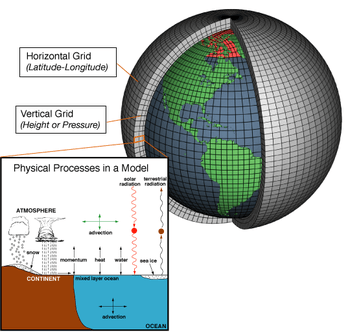
Three-dimensional (more properly four-dimensional) GCMs discretise the equations for fluid motion and integrate these forward in time. They also contain parameterisations for processes – such as convection – that occur on scales too small to be resolved directly. More sophisticated models may include representations of the carbon and other cycles.

A simple general circulation model (SGCM), a minimal GCM, consists of a dynamical core that relates material properties such as temperature to dynamical properties such as pressure and velocity. Examples are programs that solve the primitive equations, given energy input into the model, and energy dissipation in the form of scale-dependent friction, so that atmospheric waves with the highest wavenumbers are the ones most strongly attenuated. Such models may be used to study atmospheric processes within a simplified framework but are not suitable for future climate projections.

Atmospheric GCMs (AGCMs) model the atmosphere (and typically contain a land-surface model as well) and impose sea surface temperatures (SSTs). A large amount of information including model documentation is available from AMIP.^[11] They may include atmospheric chemistry.

• AGCMs consist of a dynamical core which integrates the equations of fluid motion, typically for:
  • surface pressure
  • horizontal components of velocity in layers
  • temperature and water vapor in layers
• There is generally a radiation code, split into solar/short wave and terrestrial/infra-red/long wave
• Parametrizations are used to include the effects of various processes. All modern AGCMs include parameterizations for:
  • convection
  • land surface processes, albedo and hydrology
  • cloud cover

A GCM contains a number of prognostic equations that are stepped forward in time (typically winds, temperature, moisture, and surface pressure) together with a number of diagnostic equations that are evaluated from the simultaneous values of the variables. As an example, pressure at any height can be diagnosed by applying the hydrostatic equation to the predicted surface pressure and the predicted values of temperature between the surface and the height of interest. The pressure diagnosed in this way then is used to compute the pressure gradient force in the time-dependent equation for the winds.

Oceanic GCMs (OGCMs) model the ocean (with fluxes from the atmosphere imposed) and may or may not contain a sea ice model. For example, the standard resolution of HadOM3 is 1.25 degrees in latitude and longitude, with 20 vertical levels, leading to approximately 1,500,000 variables.

Coupled atmosphere–ocean GCMs (AOGCMs) (e.g. HadCM3, GFDL CM2.X) combine the two models. They thus have the advantage of removing the need to specify fluxes across the interface of the ocean surface. These models are the basis for sophisticated model predictions of future climate, such as are discussed by the IPCC.

AOGCMs represent the pinnacle of complexity in climate models and internalise as many processes as possible. They are the only tools that could provide detailed regional predictions of future climate change. However, they are still under development. The simpler models are generally susceptible to simple analysis and their results are generally easy to understand. AOGCMs, by contrast, are often nearly as hard to analyse as the real climate system.

Model grids

The fluid equations for AGCMs are discretised using either the finite difference method or the spectral method. For finite differences, a grid is imposed on the atmosphere. The simplest grid uses constant angular grid spacing (i.e., a latitude / longitude grid), however, more sophisticated non-rectantangular grids (e.g., icosahedral) and grids of variable resolution^[12] are more often used.^[13] The "LMDz" model can be arranged to give high resolution over any given section of the planet. HadGEM1 (and other ocean models) use an ocean grid with higher resolution in the tropics to help resolve processes believed to be important for ENSO. Spectral models generally use a gaussian grid, because of the mathematics of transformation between spectral and grid-point space. Typical AGCM resolutions are between 1 and 5 degrees in latitude or longitude: the Hadley Centre model HadCM3, for example, uses 3.75 in longitude and 2.5 degrees in latitude, giving a grid of 96 by 73 points (96 x 72 for some variables); and has 19 levels in the vertical. This results in approximately 500,000 "basic" variables, since each grid point has four variables (u,v, T, Q), though a full count would give more (clouds; soil levels). HadGEM1 uses a grid of 1.875 degrees in longitude and 1.25 in latitude in the atmosphere; HiGEM, a high-resolution variant, uses 1.25 x 0.83 degrees respectively.^[14] These resolutions are lower than is typically used for weather forecasting.^[15] Ocean resolutions tend to be higher, for example HadCM3 has 6 ocean grid points per atmospheric grid point in the horizontal.

For a standard finite difference model, uniform gridlines converge towards the poles. This would lead to computational instabilities (see CFL condition) and so the model variables must be filtered along lines of latitude close to the poles. Ocean models suffer from this problem too, unless a rotated grid is used in which the North Pole is shifted onto a nearby landmass. Spectral models do not suffer from this problem. There are experiments using geodesic grids^[16] and icosahedral grids, which (being more uniform) do not have pole-problems. Another approach to solving the grid spacing problem is to deform a Cartesian cube such that it covers the surface of a sphere.^[17]

Flux buffering

Some early incarnations of AOGCMs required a somewhat ad hoc process of "flux correction" to achieve a stable climate (not all model groups used this technique). This resulted from separately prepared ocean and atmospheric models each having a different implicit flux from the other component than the other component could actually provide. If uncorrected this could lead to a dramatic drift away from observations in the coupled model. However, if the fluxes were 'corrected', the problems in the model that led to these unrealistic fluxes might be unrecognised and that might affect the model sensitivity. As a result, there has always been a strong disincentive to use flux corrections, and the vast majority of models used in the current round of the Intergovernmental Panel on Climate Change do not use them. The model improvements that now make flux corrections unnecessary are various, but include improved ocean physics, improved resolution in both atmosphere and ocean, and more physically consistent coupling between atmosphere and ocean models. Confidence in model projections is increased by the improved performance of several models that do not use flux adjustment. These models now maintain stable, multi-century simulations of surface climate that are considered to be of sufficient quality to allow their use for climate change projections.^[18]

Convection

Moist convection causes the release of latent heat and is important to the Earth's energy budget. Convection occurs on too small a scale to be resolved by climate models, and hence it must be parameterized. This has been done since the earliest days of climate modelling, in the 1950s. Akio Arakawa did much of the early work, and variants of his scheme are still used,^[19] although there are a variety of different schemes now in use.^[20][21][22] Clouds are typically parametrized, not because their physical processes are poorly understood, but because they occur on a scale smaller than the resolved scale of most GCMs. The causes and effects of their small scale actions on the large scale are represented by large scale parameters, hence "parameterization". The fact that cloud processes are not perfectly parameterized is due in part to a lack of understanding of clouds, but not due to some inherent shortcoming of the method.^[23]

Output variables

Most models include software to diagnose a wide range of variables for comparison with observations or study of processes within the atmosphere. An example is the 1.5-metre temperature, which is the standard height for near-surface observations of air temperature. This temperature is not directly predicted from the model but is deduced from the surface and lowest-model-layer temperatures. Other software is used for creating plots and animations.

Projections of future climate change

Projected annual mean surface air temperature from 1970-2100, based on SRES emissions scenario A1B, using the NOAA GFDL CM2.1 climate model (credit: NOAA Geophysical Fluid Dynamics Laboratory).^[24]

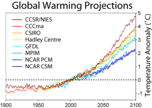
Coupled ocean–atmosphere GCMs use transient climate simulations to project/predict future temperature changes under various scenarios. These can be idealised scenarios (most commonly, CO₂ increasing at 1%/yr) or more realistic (usually the "IS92a" or more recently the SRES scenarios). Which scenarios should be considered most realistic is currently uncertain, as the projections of future CO₂ (and sulphate) emission are themselves uncertain.

The 2001 IPCC Third Assessment Report figure 9.3 shows the global mean response of 19 different coupled models to an idealised experiment in which CO₂ is increased at 1% per year.^[25] Figure 9.5 shows the response of a smaller number of models to more realistic forcing. For the 7 climate models shown there, the temperature change to 2100 varies from 2 to 4.5 °C with a median of about 3 °C.

Future scenarios do not include unknowable events – for example, volcanic eruptions or changes in solar forcing. These effects are believed to be small in comparison to greenhouse gas (GHG) forcing in the long term, but large volcanic eruptions, for example, are known to exert a temporary cooling effect.

Human emissions of GHGs are an external input to the models, although it would be possible to couple in an economic model to provide these as well. Atmospheric GHG levels are usually supplied as an input, though it is possible to include a carbon cycle model including land vegetation and oceanic processes to calculate GHG levels.

Emissions scenarios

Projected change in annual mean surface air temperature from the late 20th century to the middle 21st century, based on SRES emissions scenario A1B (credit: NOAA Geophysical Fluid Dynamics Laboratory).^[24]

For the six SRES marker scenarios, IPCC (2007:7–8) gave a "best estimate" of global mean temperature increase (2090–2099 relative to the period 1980–99) that ranged from 1.8 °C to 4.0 °C.^[26] Over the same time period, the "likely" range (greater than 66% probability, based on expert judgement) for these scenarios was for a global mean temperature increase of between 1.1 and 6.4 °C.^[26]

Pope (2008) described a study where climate change projections were made using several different emission scenarios.^[27] In a scenario where global emissions start to decrease by 2010 and then decline at a sustained rate of 3% per year, the likely global average temperature increase was predicted to be 1.7 °C above pre-industrial levels by 2050, rising to around 2 °C by 2100. In a projection designed to simulate a future where no efforts are made to reduce global emissions, the likely rise in global average temperature was predicted to be 5.5 °C by 2100. A rise as high as 7 °C was thought possible but less likely.

Sokolov et al. (2009) examined a scenario designed to simulate a future where there is no policy to reduce emissions. In their integrated model, this scenario resulted in a median warming over land (2090–99 relative to the period 1980–99) of 5.1 °C. Under the same emissions scenario but with different modeling of the future climate, the predicted median warming was 4.1 °C.^[28]

Accuracy of models that predict global warming

SST errors in HadCM3

North American precipitation from various models.

Temperature predictions from some climate models assuming the SRES A2 emissions scenario.

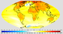
AOGCMs represent the pinnacle of complexity in climate models and internalise as many processes as possible. However, they are still under development and uncertainties remain. They may be coupled to models of other processes, such as the carbon cycle, so as to better model feedback effects. Most recent simulations show "plausible" agreement with the measured temperature anomalies over the past 150 years, when forced by observed changes in greenhouse gases and aerosols, and better agreement is achieved when both natural and man-made forcings are included.^[29][30]

No model – whether a wind-tunnel model for designing aircraft, or a climate model for projecting global warming – perfectly reproduces the system being modeled. Such inherently imperfect models may nevertheless produce useful results. In this context, GCMs are capable of reproducing the general features of the observed global temperature over the past century.^[29]

A debate over how to reconcile climate model predictions that upper air (tropospheric) warming should be greater than surface warming, with observations some of which appeared to show otherwise^[31] now appears to have been resolved in favour of the models, following revisions to the data: see satellite temperature record.

The effects of clouds are a significant area of uncertainty in climate models. Clouds have competing effects on the climate. One of the roles that clouds play in climate is in cooling the surface by reflecting sunlight back into space; another is warming by increasing the amount of infrared radiation emitted from the atmosphere to the surface.^[32] In the 2001 IPCC report on climate change, the possible changes in cloud cover were highlighted as one of the dominant uncertainties in predicting future climate change;^[33] see also^[34]

Thousands of climate researchers around the world use climate models to understand the climate system. There are thousands of papers published about model-based studies in peer-reviewed journals – and a part of this research is work improving the models. Improvement has been difficult but steady (most obviously, state of the art AOGCMs no longer require flux correction), and progress has sometimes led to discovering new uncertainties.

In 2000, a comparison between measurements and dozens of GCM simulations of ENSO-driven tropical precipitation, water vapor, temperature, and outgoing longwave radiation found similarity between measurements and simulation of most factors. However the simulated change in precipitation was about one-fourth less than what was observed. Errors in simulated precipitation imply errors in other processes, such as errors in the evaporation rate that provides moisture to create precipitation. The other possibility is that the satellite-based measurements are in error. Either indicates progress is required in order to monitor and predict such changes.^[35]

A more complete discussion of climate models is provided in the IPCC's Third Assessment Report.^[36]

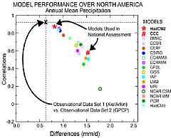
• The model mean exhibits good agreement with observations.
• The individual models often exhibit worse agreement with observations.
• Many of the non-flux adjusted models suffered from unrealistic climate drift up to about 1 °C/century in global mean surface temperature.
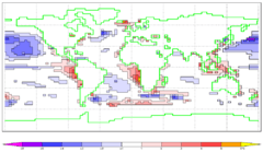
• The errors in model-mean surface air temperature rarely exceed 1 °C over the oceans and 5 °C over the continents; precipitation and sea level pressure errors are relatively greater but the magnitudes and patterns of these quantities are recognisably similar to observations.
• Surface air temperature is particularly well simulated, with nearly all models closely matching the observed magnitude of variance and exhibiting a correlation > 0.95 with the observations.
• Simulated variance of sea level pressure and precipitation is within ±25% of observed.
• All models have shortcomings in their simulations of the present day climate of the stratosphere, which might limit the accuracy of predictions of future climate change.
  • There is a tendency for the models to show a global mean cold bias at all levels.
  • There is a large scatter in the tropical temperatures.
  • The polar night jets in most models are inclined poleward with height, in noticeable contrast to an equatorward inclination of the observed jet.
  • There is a differing degree of separation in the models between the winter sub-tropical jet and the polar night jet.
• For nearly all models the r.m.s. error in zonal- and annual-mean surface air temperature is small compared with its natural variability.
  • There are problems in simulating natural seasonal variability. ( 2000)
    • In flux-adjusted models, seasonal variations are simulated to within 2 K of observed values over the oceans. The corresponding average over non-flux-adjusted models shows errors up to about 6 K in extensive ocean areas.
    • Near-surface land temperature errors are substantial in the average over flux-adjusted models, which systematically underestimates (by about 5 K) temperature in areas of elevated terrain. The corresponding average over non-flux-adjusted models forms a similar error pattern (with somewhat increased amplitude) over land.
    • In Southern Ocean mid-latitudes, the non-flux-adjusted models overestimate the magnitude of January-minus-July temperature differences by ~5 K due to an overestimate of summer (January) near-surface temperature. This error is common to five of the eight non-flux-adjusted models.
    • Over Northern Hemisphere mid-latitude land areas, zonal mean differences between July and January temperatures simulated by the non-flux-adjusted models show a greater spread (positive and negative) about observed values than results from the flux-adjusted models.
    • The ability of coupled GCMs to simulate a reasonable seasonal cycle is a necessary condition for confidence in their prediction of long-term climatic changes (such as global warming), but it is not a sufficient condition unless the seasonal cycle and long-term changes involve similar climatic processes.
• Coupled climate models do not simulate with reasonable accuracy clouds and some related hydrological processes (in particular those involving upper tropospheric humidity). Problems in the simulation of clouds and upper tropospheric humidity, remain worrisome because the associated processes account for most of the uncertainty in climate model simulations of anthropogenic change.

The precise magnitude of future changes in climate is still uncertain;^[37] for the end of the 21st century (2071 to 2100), for SRES scenario A2, the change of global average SAT change from AOGCMs compared with 1961 to 1990 is +3.0 °C (4.8 °F) and the range is +1.3 to +4.5 °C (+2 to +7.2 °F).

In the IPCC's Fifth Assessment Report, it was stated that there was "...very high confidence that models reproduce the general features of the global-scale annual mean surface temperature increase over the historical period." However, the report also observed that the rate of warming over the period 1998-2012 was lower than that predicted by 111 out of 114 Coupled Model Intercomparison Project climate models.^[38]

Relation to weather forecasting

The global climate models used for climate projections are very similar in structure to (and often share computer code with) numerical models for weather prediction but are nonetheless logically distinct.

Most weather forecasting is done on the basis of interpreting the output of numerical model results. Since forecasts are short—typically a few days or a week—such models do not usually contain an ocean model but rely on imposed SSTs. They also require accurate initial conditions to begin the forecast—typically these are taken from the output of a previous forecast, with observations blended in. Because the results are needed quickly the predictions must be run in a few hours; but because they only need to cover a week of real time these predictions can be run at higher resolution than in climate mode. Currently the ECMWF runs at 40 km (25 mi) resolution^[39] as opposed to the 100-to-200 km (62-to-124 mi) scale used by typical climate models. Often nested models are run forced by the global models for boundary conditions, to achieve higher local resolution: for example, the Met Office runs a mesoscale model with an 11 km (6.8 mi) resolution^[40] covering the UK, and various agencies in the U.S. also run nested models such as the NGM and NAM models. Like most global numerical weather prediction models such as the GFS, global climate models are often spectral models^[41] instead of grid models. Spectral models are often used for global models because some computations in modeling can be performed faster thus reducing the time needed to run the model simulation.

Computations involved

Climate models use quantitative methods to simulate the interactions of the atmosphere, oceans, land surface, and ice. They are used for a variety of purposes from study of the dynamics of the climate system to projections of future climate.

All climate models take account of incoming energy as short wave electromagnetic radiation, chiefly visible and short-wave (near) infrared, as well as outgoing energy as long wave (far) infrared electromagnetic radiation from the earth. Any imbalance results in a change in temperature.

The most talked-about models of recent years have been those relating temperature to emissions of carbon dioxide (see greenhouse gas). These models project an upward trend in the surface temperature record, as well as a more rapid increase in temperature at higher altitudes.^[42]

Three (or more properly, four since time is also considered) dimensional GCM's discretise the equations for fluid motion and energy transfer and integrate these over time. They also contain parametrisations for processes—such as convection—that occur on scales too small to be resolved directly.

Atmospheric GCMs (AGCMs) model the atmosphere and impose sea surface temperatures as boundary conditions. Coupled atmosphere-ocean GCMs (AOGCMs, e.g. HadCM3, EdGCM, GFDL CM2.X, ARPEGE-Climat^[43]) combine the two models.

Models can range from relatively simple to quite complex:

• A simple radiant heat transfer model that treats the earth as a single point and averages outgoing energy
• this can be expanded vertically (radiative-convective models), or horizontally
• finally, (coupled) atmosphere–ocean–sea ice global climate models discretise and solve the full equations for mass and energy transfer and radiant exchange.

This is not a full list; for example "box models" can be written to treat flows across and within ocean basins. Furthermore, other types of modelling can be interlinked, such as land use, allowing researchers to predict the interaction between climate and ecosystems.

Other climate models

Earth-system models of intermediate complexity (EMICs)

Depending on the nature of questions asked and the pertinent time scales, there are, on the one extreme, conceptual, more inductive models, and, on the other extreme, general circulation models operating at the highest spatial and temporal resolution currently feasible. Models of intermediate complexity bridge the gap. One example is the Climber-3 model. Its atmosphere is a 2.5-dimensional statistical-dynamical model with 7.5° × 22.5° resolution and time step of 1/2 a day; the ocean is MOM-3 (Modular Ocean Model) with a 3.75° × 3.75° grid and 24 vertical levels.

• http://www.pik-potsdam.de/emics/

Radiative-convective models (RCM)

One-dimensional, radiative-convective models were used to verify basic climate assumptions in the '80s and '90s.^[44]

Climate modelers

A climate modeler is a person who designs, develops, implements, tests, maintains or exploits climate models. There are three major types of institutions where a climate modeller may be found:

• In a national meteorological service. Most national weather services have at least a climatology section.
• In a university. Departments that may have climate modellers on staff include atmospheric sciences, meteorology, climatology, or geography, amongst others.
• In national or international research laboratories specialising in this field, such as the National Center for Atmospheric Research (NCAR, in Boulder, Colorado, USA), the Geophysical Fluid Dynamics Laboratory (GFDL, in Princeton, New Jersey), the Hadley Centre for Climate Prediction and Research (in Exeter, UK), the Max Planck Institute for Meteorology in Hamburg, Germany, or the Institut Pierre-Simon Laplace (IPSL in Paris, France). The World Climate Research Programme (WCRP), hosted by the World Meteorological Organization (WMO), coordinates research activities on climate modeling worldwide.

See also

• Atmospheric Model Intercomparison Project (AMIP)
• Atmospheric Radiation Measurement (ARM) (in the US)
• Earth Simulator
• Global Environmental Multiscale Model
• Intermediate General Circulation Model
• NCAR
• Prognostic variable

References

• IPCC AR4 SYR (2007), Core Writing Team; Pachauri, R.K; and Reisinger, A., ed., Climate Change 2007: Synthesis Report (SYR), Contribution of Working Groups I, II and III to the Fourth Assessment Report (AR4) of the Intergovernmental Panel on Climate Change, Geneva, Switzerland: IPCC, ISBN 92-9169-122-4 .

Further reading

• Ian Roulstone and John Norbury (2013). Invisible in the Storm: the role of mathematics in understanding weather. Princeton University Press. 

External links

• IPCC AR5, Evaluation of Climate Models
• Media from GFDL's CCVP Group. Includes videos, animations, podcasts and transcripts on climate models.
• GFDL's Flexible Modeling System containing code for the climate models.
• Program for climate model diagnosis and intercomparison (PCMDI/CMIP)
• National Operational Model Archive and Distribution System (NOMADS)
• Hadley Centre for Climate Prediction and Research – model info
• NCAR/UCAR Community Climate System Model (CESM)
• Climate prediction, community modeling
• NASA/GISS, primary research GCM model
• EDGCM/NASA: Educational Global Climate Modeling
• NOAA/GFDL

References

- ↑ "The First Climate Model". NOAA. Retrieved 12 January 2014.
- ↑ 2.0 2.1 ": The First Climate Model". NOAA 200th Celebration. 2007. Retrieved 20 April 2010.
- ↑ Phillips, Norman A. (April 1956). "The general circulation of the atmosphere: a numerical experiment". Quarterly Journal of the Royal Meteorological Society 82 (352): 123–154. Bibcode:1956QJRMS..82..123P. doi:10.1002/qj.49708235202.
- ↑ Cox, John D. (2002). Storm Watchers. John Wiley & Sons, Inc. p. 210. ISBN 0-471-38108-X.
- ↑ 5.0 5.1 Lynch, Peter (2006). "The ENIAC Integrations". The Emergence of Numerical Weather Prediction. Cambridge University Press. pp. 206–208. ISBN 978-0-521-85729-1.
- ↑ Collins, William D. et al. (June 2004). "Description of the NCAR Community Atmosphere Model (CAM 3.0)". University Corporation for Atmospheric Research. Retrieved 3 January 2011.
- ↑ Xue, Yongkang and Michael J. Fennessey (20 March 1996). "Impact of vegetation properties on U.S. summer weather prediction". Journal of Geophysical Research (American Geophysical Union) 101 (D3): 7419. Bibcode:1996JGR...101.7419X. doi:10.1029/95JD02169. Retrieved 6 January 2011.
- ↑ McGuffie, K. and A. Henderson-Sellers (2005). A climate modelling primer. John Wiley and Sons. p. 188. ISBN 978-0-470-85751-9.
- ↑ Allen, Jeannie (February 2004). "Tango in the Atmosphere: Ozone and Climate Change". NASA Earth Observatory. Retrieved 20 April 2010.
- ↑ Ken, Richard A (13 April 2001). "Global Warming: Rising Global Temperature, Rising Uncertainty". Science 292 (5515): 192–194. doi:10.1126/science.292.5515.192. PMID 11305301. Retrieved 20 April 2010.
- ↑ "Atmospheric Model Intercomparison Project". The Program for Climate Model Diagnosis and Intercomparison, Lawrence Livermore National Laboratory. Retrieved 21 April 2010.
- ↑ C. Jablonowski , M. Herzog , J. E. Penner , R. C. Oehmke , Q. F. Stout , B. van Leer, January 1960.5091 "Adaptive Grids for Weather and Climate Models" (2004). See also Christiane Jablonowski, Adaptive Mesh Refinement (AMR) for Weather and Climate Models page (Retrieved 24 July 2010)
- ↑ NCAR Command Language documentation: Non-uniform grids that NCL can contour (Retrieved 24 July 2010)
- ↑ "High Resolution Global Environmental Modelling (HiGEM) home page". Natural Environment Research Council and Met Office. 18 May 2004. Retrieved 5 October 2010.
- ↑ "Mesoscale modelling". Retrieved 5 October 2010.
- ↑ "Climate Model Will Be First To Use A Geodesic Grid". Daly University Science News. 24 September 2001. Retrieved 3 May 2011.
- ↑ "Gridding the sphere". MIT GCM. Retrieved 9 September 2010.
- ↑ "IPCC Third Assessment Report - Climate Change 2001 - Complete online versions". IPCC. Retrieved 12 January 2014.
- ↑ "Arakawa's Computation Device". Aip.org. Retrieved 2012-02-18.
- ↑ "COLA Report 27". Grads.iges.org. 1996-07-01. Retrieved 2012-02-18.
- ↑ "Table 2-10". Pcmdi.llnl.gov. Retrieved 2012-02-18.
- ↑ "Table of Rudimentary CMIP Model Features". Rainbow.llnl.gov. 2004-12-02. Retrieved 2012-02-18.
- ↑ "General Circulation Models of the Atmosphere". Aip.org. Retrieved 2012-02-18.
- ↑ 24.0 24.1 NOAA Geophysical Fluid Dynamics Laboratory (GFDL) (9 October 2012), NOAA GFDL Climate Research Highlights Image Gallery: Patterns of Greenhouse Warming, NOAA GFDL
- ↑ "Climate Change 2001: The Scientific Basis". Grida.no. Retrieved 2012-02-18.
- ↑ 26.0 26.1 "Summary for Policymakers", 3. Projected climate change and its impacts Missing or empty