Gamma distribution
Probability density function | ||
Cumulative distribution function | ||
| Parameters |
| |
|---|---|---|
| Support |  |
|
| Probability density function (pdf) | 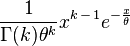 |
 |
| Cumulative distribution function (CDF) | 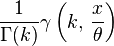 |
 |
| Mean | ![\scriptstyle \mathbf{E}[ X] = k \theta](../I/m/2ef7149067051a214ef8e06fcda59c69.png) ![\scriptstyle \mathbf{E}[\ln X] = \psi(k) +\ln(\theta)](../I/m/8da978fa9d16f099aff1689d80353243.png) (see digamma function) |
![\scriptstyle\mathbf{E}[ X] = \frac{\alpha}{\beta}](../I/m/8f86054b1b623c69ba08ceec928f751a.png) ![\scriptstyle \mathbf{E}[\ln X] = \psi(\alpha) -\ln(\beta)](../I/m/1ed332352249e04f14d31bd39b1c69d0.png) (see digamma function) |
| Median | No simple closed form | No simple closed form |
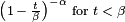
| Mode |  |
 |
| Variance | ![\scriptstyle\operatorname{Var}[ X] = k \theta^2](../I/m/aaffe1c9d35387fc3a4ca41b8930433d.png) ![\scriptstyle\operatorname{Var}[\ln X] = \psi_1(k)](../I/m/f2eb1c6c9275c0bb96e92cf5412a6696.png) (see trigamma function) |
![\scriptstyle \operatorname{Var}[ X] = \frac{\alpha}{\beta^2}](../I/m/f703b1c204d5b9cdb6fc527c0cc8cfab.png) ![\scriptstyle\operatorname{Var}[\ln X] = \psi_1(\alpha)](../I/m/f94b50c53729a19c515138c7756bcb15.png) (see trigamma function) |
| Skewness |  |
 |
| Excess kurtosis |  |
 |
| Entropy | ![\scriptstyle \begin{align}
\scriptstyle k &\scriptstyle \,+\, \ln\theta \,+\, \ln[\Gamma(k)]\\
\scriptstyle &\scriptstyle \,+\, (1 \,-\, k)\psi(k)
\end{align}](../I/m/439ae7b561921950377e3858363abdfd.png) |
![\scriptstyle \begin{align}
\scriptstyle \alpha &\scriptstyle \,-\, \ln \beta \,+\, \ln[\Gamma(\alpha)]\\
\scriptstyle &\scriptstyle \,+\, (1 \,-\, \alpha)\psi(\alpha)
\end{align}](../I/m/8a54a178f2bae2a40f0869701fa2a29e.png) |
| Moment-generating function (mgf) | 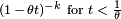 |
 |
| Characteristic function |  |
 |
In probability theory and statistics, the gamma distribution is a two-parameter family of continuous probability distributions. The common exponential distribution and chi-squared distribution are special cases of the gamma distribution. There are three different parametrizations in common use:
- With a shape parameter k and a scale parameter θ.
- With a shape parameter α = k and an inverse scale parameter β = 1/θ, called a rate parameter.
- With a shape parameter k and a mean parameter μ = k/β.
In each of these three forms, both parameters are positive real numbers.
The parameterization with k and θ appears to be more common in econometrics and certain other applied fields, where e.g. the gamma distribution is frequently used to model waiting times. For instance, in life testing, the waiting time until death is a random variable that is frequently modeled with a gamma distribution.[1]
The parameterization with α and β is more common in Bayesian statistics, where the gamma distribution is used as a conjugate prior distribution for various types of inverse scale (aka rate) parameters, such as the λ of an exponential distribution or a Poisson distribution[2] – or for that matter, the β of the gamma distribution itself. (The closely related inverse gamma distribution is used as a conjugate prior for scale parameters, such as the variance of a normal distribution.)
If k is an integer, then the distribution represents an Erlang distribution; i.e., the sum of k independent exponentially distributed random variables, each of which has a mean of θ (which is equivalent to a rate parameter of 1/θ).
The gamma distribution is the maximum entropy probability distribution for a random variable X for which E[X] = kθ = α/β is fixed and greater than zero, and E[ln(X)] = ψ(k) + ln(θ) = ψ(α) − ln(β) is fixed (ψ is the digamma function).[3]
Characterization using shape k and scale θ
A random variable X that is gamma-distributed with shape k and scale θ is denoted by

Probability density function

The probability density function using the shape-scale parametrization is
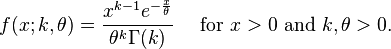
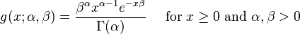
Here Γ(k) is the gamma function evaluated at k.
Cumulative distribution function
The cumulative distribution function is the regularized gamma function:
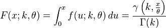
where γ(k, x/θ) is the lower incomplete gamma function.
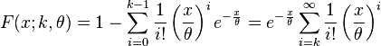
It can also be expressed as follows, if k is a positive integer (i.e., the distribution is an Erlang distribution):[4]
Characterization using shape α and rate β
Alternatively, the gamma distribution can be parameterized in terms of a shape parameter α = k and an inverse scale parameter β = 1/θ, called a rate parameter. A random variable X that is gamma-distributed with shape α and rate β is denoted

Probability density function
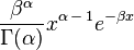
The corresponding density function in the shape-rate parametrization is
Both parametrizations are common because either can be more convenient depending on the situation.
Cumulative distribution function
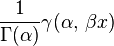
The cumulative distribution function is the regularized gamma function:
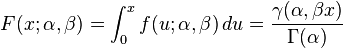
where γ(α, βx) is the lower incomplete gamma function.
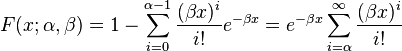
If α is a positive integer (i.e., the distribution is an Erlang distribution), the cumulative distribution function has the following series expansion:[4]
Properties
Skewness
The skewness is equal to  , it depends only on the shape parameter (k) and approaches a normal distribution when k is large (approximately when k > 10).
Median calculation
Unlike the mode and the mean which have readily calculable formulas based on the parameters, the median does not have an easy closed form equation. The median for this distribution is defined as the value ν such that
A formula for approximating the median for any gamma distribution, when the mean is known, has been derived based on the fact that the ratio μ/(μ − ν) is approximately a linear function of k when k ≥ 1.[5] The approximation formula is
where  is the mean.
Summation
If Xi has a Gamma(ki, θ) distribution for i = 1, 2, ..., N (i.e., all distributions have the same scale parameter θ), then
provided all Xi are independent.
For the cases where the Xi are independent but have different scale parameters see Mathai (1982) and Moschopoulos (1984).
The gamma distribution exhibits infinite divisibility.
Scaling
If
then, for any c > 0,
Indeed, we know that if X is an exponential r.v. with rate \lambda then c X is an exponential r.v. with rate \lambda / c; the same thing is valid with Gamma variates (and this can be checked using the moment-generating function, see, e.g., these notes, 10.4-(ii)): multiplication by a positive constant c divides the rate (or, equivalently, multiplies the scale).
Exponential family
The gamma distribution is a two-parameter exponential family with natural parameters k − 1 and −1/θ (equivalently, α − 1 and −β), and natural statistics X and ln(X).
If the shape parameter k is held fixed, the resulting one-parameter family of distributions is a natural exponential family.
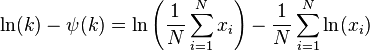
Logarithmic expectation
One can show that
![\mathbf{E}[\ln(X)] = \psi(\alpha) - \ln(\beta)](../I/m/98e327a27c1e59d2b49005cd9b51af93.png)
or equivalently,
![\mathbf{E}[\ln(X)] = \psi(k) + \ln(\theta)](../I/m/20337bf8e4599e121f37ad59eb22b25a.png)
where ψ is the digamma function.
This can be derived using the exponential family formula for the moment generating function of the sufficient statistic, because one of the sufficient statistics of the gamma distribution is ln(x).
Information entropy
The information entropy is
![\operatorname{H}(X) = \mathbf{E}[-\ln(p(X))] = \mathbf{E}[-\alpha\ln(\beta) + \ln(\Gamma(\alpha)) - (\alpha-1)\ln(X) + \beta X] = \alpha - \ln(\beta) + \ln(\Gamma(\alpha)) + (1-\alpha)\psi(\alpha).](../I/m/6ae9e4d1b1097ee9af115d1bf0b3b908.png)
In the k, θ parameterization, the information entropy is given by

Kullback–Leibler divergence

The Kullback–Leibler divergence (KL-divergence), of Gamma(αp, βp) ("true" distribution) from Gamma(αq, βq) ("approximating" distribution) is given by[6]

Written using the k, θ parameterization, the KL-divergence of Gamma(kp, θp) from Gamma(kq, θq) is given by

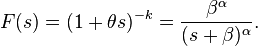
Laplace transform
The Laplace transform of the gamma PDF is
Differential equation
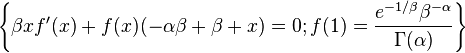
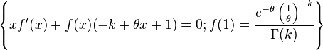
Parameter estimation
Maximum likelihood estimation
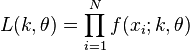
The likelihood function for N iid observations (x1, ..., xN) is
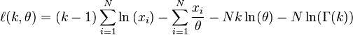
from which we calculate the log-likelihood function
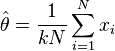
Finding the maximum with respect to θ by taking the derivative and setting it equal to zero yields the maximum likelihood estimator of the θ parameter:
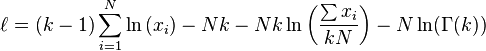
Substituting this into the log-likelihood function gives
Finding the maximum with respect to k by taking the derivative and setting it equal to zero yields
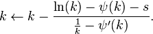
There is no closed-form solution for k. The function is numerically very well behaved, so if a numerical solution is desired, it can be found using, for example, Newton's method. An initial value of k can be found either using the method of moments, or using the approximation
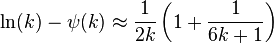
If we let
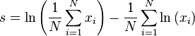
then k is approximately
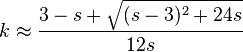
which is within 1.5% of the correct value.[7] An explicit form for the Newton–Raphson update of this initial guess is:[8]
Bayesian minimum mean squared error
With known k and unknown θ, the posterior density function for theta (using the standard scale-invariant prior for θ) is
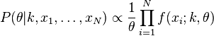
Denoting
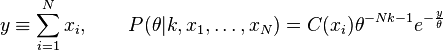
Integration over θ can be carried out using a change of variables, revealing that 1/θ is gamma-distributed with parameters α = Nk, β = y.

The moments can be computed by taking the ratio (m by m = 0)
![\mathbf{E} [x^m] = \frac {\Gamma (Nk - m)} {\Gamma(Nk)} y^m](../I/m/67cbb75df262c485542f564800709dad.png)
which shows that the mean ± standard deviation estimate of the posterior distribution for θ is
Generating gamma-distributed random variables
Given the scaling property above, it is enough to generate gamma variables with θ = 1 as we can later convert to any value of β with simple division.
Suppose we wish to generate random variables from Gamma(n+δ,1), where n is a non-negative integer and 0 < δ < 1. Using the fact that a Gamma(1, 1) distribution is the same as an Exp(1) distribution, and noting the method of generating exponential variables, we conclude that if U is uniformly distributed on (0, 1], then −ln(U) is distributed Gamma(1, 1). Now, using the "α-addition" property of gamma distribution, we expand this result:
where Uk are all uniformly distributed on (0, 1] and independent. All that is left now is to generate a variable distributed as Gamma(δ, 1) for 0 < δ < 1 and apply the "α-addition" property once more. This is the most difficult part.
Random generation of gamma variates is discussed in detail by Devroye,[9] noting that none are uniformly fast for all shape parameters. For small values of the shape parameter, the algorithms are often not valid.[10] For arbitrary values of the shape parameter, one can apply the Ahrens and Dieter[11] modified acceptance–rejection method Algorithm GD (shape k ≥ 1), or transformation method[12] when 0 < k < 1. Also see Cheng and Feast Algorithm GKM 3[13] or Marsaglia's squeeze method.[14]
The following is a version of the Ahrens-Dieter acceptance–rejection method:[11]
- Let m be 1.
- Generate V3m−2, V3m−1 and V3m as independent uniformly distributed on (0, 1] variables.
- If
 , where
  , then go to step 4, else go to step 5.
 - Let
 . Go to step 6.
 - Let
 .
. - If
 , then increment m and go to step 2.
 - Assume ξ = ξm to be the realization of Γ(δ, 1).
A summary of this is
where
-
 is the integral part of k,
 - ξ has been generated using the algorithm above with δ = {k} (the fractional part of k),
- Uk and Vl are distributed as explained above and are all independent.
While the above approach is technically correct, Devroye notes that it is linear in the value of k and in general is not a good choice. Instead he recommends using either rejection-based or table-based methods, depending on context.[15]
Related distributions
Conjugate prior
In Bayesian inference, the gamma distribution is the conjugate prior to many likelihood distributions: the Poisson, exponential, normal (with known mean), Pareto, gamma with known shape σ, inverse gamma with known shape parameter, and Gompertz with known scale parameter.
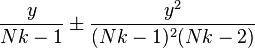
The gamma distribution's conjugate prior is:[16]
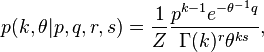
where Z is the normalizing constant, which has no closed-form solution. The posterior distribution can be found by updating the parameters as follows:
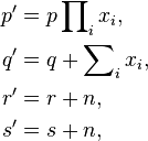
where n is the number of observations, and xi is the ith observation.
Compound gamma
If the shape parameter of the gamma distribution is known, but the inverse-scale parameter is unknown, then a gamma distribution for the inverse-scale forms a conjugate prior. The compound distribution, which results from integrating out the inverse-scale, has a closed form solution, known as the compound gamma distribution.[17]
Others
- If X ~ Gamma(1, 1/λ) (shape -scale parametrization), then X has an exponential distribution with rate parameter λ.
- If X ~ Gamma(ν/2, 2), then X is identical to χ2(ν), the chi-squared distribution with ν degrees of freedom. Conversely, if Q ~ χ2(ν) and c is a positive constant, then cQ ~ Gamma(ν/2, 2c).
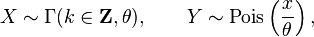
- If k is an integer, the gamma distribution is an Erlang distribution and is the probability distribution of the waiting time until the kth "arrival" in a one-dimensional Poisson process with intensity 1/θ. If
- then
- If X has a Maxwell–Boltzmann distribution with parameter a, then
 .
.
- If X ~ Gamma(k, θ), then
 follows a generalized gamma distribution with parameters p = 2, d = 2k, and
  .
. - If X ~ Gamma(k, θ), then 1/X ~ Inv-Gamma(k, θ−1) (see Inverse-gamma distribution for derivation).
- If X ~ Gamma(α, θ) and Y ~ Gamma(β, θ) are independently distributed, then X/(X + Y) has a beta distribution with parameters α and β.
- If Xi ~ Gamma(αi, 1) are independently distributed, then the vector (X1/S, ..., Xn/S), where S = X1 + ... + Xn, follows a Dirichlet distribution with parameters α1, ..., αn.
- For large k the gamma distribution converges to Gaussian distribution with mean μ = kθ and variance σ2 = kθ2.
- The gamma distribution is the conjugate prior for the precision of the normal distribution with known mean.
- The Wishart distribution is a multivariate generalization of the gamma distribution (samples are positive-definite matrices rather than positive real numbers).
- The gamma distribution is a special case of the generalized gamma distribution, the generalized integer gamma distribution, and the generalized inverse Gaussian distribution.
- Among the discrete distributions, the negative binomial distribution is sometimes considered the discrete analogue of the Gamma distribution.
- Tweedie distributions – the gamma distribution is a member of the family of Tweedie exponential dispersion models.
Applications
The gamma distribution has been used to model the size of insurance claims[18] and rainfalls.[19] This means that aggregate insurance claims and the amount of rainfall accumulated in a reservoir are modelled by a gamma process. The gamma distribution is also used to model errors in multi-level Poisson regression models, because the combination of the Poisson distribution and a gamma distribution is a negative binomial distribution.
In neuroscience, the gamma distribution is often used to describe the distribution of inter-spike intervals.[20] Although in practice the gamma distribution often provides a good fit, there is no underlying biophysical motivation for using it.
In bacterial gene expression, the copy number of a constitutively expressed protein often follows the gamma distribution, where the scale and shape parameter are, respectively, the mean number of bursts per cell cycle and the mean number of protein molecules produced by a single mRNA during its lifetime.[21]
In genomics, the gamma distribution was applied in peak calling step (i.e. in recognition of signal) in ChIP-chip[22] and ChIP-seq[23] data analysis.
The gamma distribution is widely used as a conjugate prior in Bayesian statistics. It is the conjugate prior for the precision (i.e. inverse of the variance) of a normal distribution. It is also the conjugate prior for the exponential distribution.
Notes
- ↑ See Hogg and Craig (1978, Remark 3.3.1) for an explicit motivation
- ↑ Scalable Recommendation with Poisson Factorization, Prem Gopalan, Jake M. Hofman, David Blei, arXiv.org 2014
- ↑ Park, Sung Y.; Bera, Anil K. (2009). "Maximum entropy autoregressive conditional heteroskedasticity model" (PDF). Journal of Econometrics (Elsevier): 219–230. doi:10.1016/j.jeconom.2008.12.014. Retrieved 2011-06-02.
- ↑ 4.0 4.1 Papoulis, Pillai, Probability, Random Variables, and Stochastic Processes, Fourth Edition
- ↑ Banneheka BMSG, Ekanayake GEMUPD (2009) "A new point estimator for the median of gamma distribution". Viyodaya J Science, 14:95–103
- ↑ W.D. Penny, [www.fil.ion.ucl.ac.uk/~wpenny/publications/densities.ps KL-Divergences of Normal, Gamma, Dirichlet, and Wishart densities]
- ↑ Minka, Thomas P. (2002) "Estimating a Gamma distribution". http://research.microsoft.com/en-us/um/people/minka/papers/minka-gamma.pdf
- ↑ Choi, S.C.; Wette, R. (1969) "Maximum Likelihood Estimation of the Parameters of the Gamma Distribution and Their Bias", Technometrics, 11(4) 683–690
- ↑ Luc Devroye (1986). Non-Uniform Random Variate Generation. New York: Springer-Verlag. See Chapter 9, Section 3, pages 401–428.
- ↑ Devroye (1986), p. 406.
- ↑ 11.0 11.1 Ahrens, J. H. and Dieter, U. (1982). Generating gamma variates by a modified rejection technique. Communications of the ACM, 25, 47–54. Algorithm GD, p. 53.
- ↑ Ahrens, J. H.; Dieter, U. (1974). "Computer methods for sampling from gamma, beta, Poisson and binomial distributions". Computing 12: 223–246. doi:10.1007/BF02293108. CiteSeerX: 10
.1 ..1 .93 .3828 - ↑ Cheng, R.C.H., and Feast, G.M. Some simple gamma variate generators. Appl. Stat. 28 (1979), 290–295.
- ↑ Marsaglia, G. The squeeze method for generating gamma variates. Comput, Math. Appl. 3 (1977), 321–325.
- ↑ Luc Devroye (1986). Non-Uniform Random Variate Generation. New York: Springer-Verlag. See Chapter 9, Section 3, pages 401–428.
- ↑ Fink, D. 1995 A Compendium of Conjugate Priors. In progress report: Extension and enhancement of methods for setting data quality objectives. (DOE contract 95‑831).
- ↑ Dubey, Satya D. (December 1970). "Compound gamma, beta and F distributions". Metrika 16: 27–31. doi:10.1007/BF02613934.
- ↑ p. 43, Philip J. Boland, Statistical and Probabilistic Methods in Actuarial Science, Chapman & Hall CRC 2007
- ↑ Aksoy, H. (2000) "Use of Gamma Distribution in Hydrological Analysis", Turk J. Engin Environ Sci, 24, 419 – 428.
- ↑ J. G. Robson and J. B. Troy, "Nature of the maintained discharge of Q, X, and Y retinal ganglion cells of the cat", J. Opt. Soc. Am. A 4, 2301–2307 (1987)
- ↑ N. Friedman, L. Cai and X. S. Xie (2006) "Linking stochastic dynamics to population distribution: An analytical framework of gene expression", Phys. Rev. Lett. 97, 168302.
- ↑ DJ Reiss, MT Facciotti and NS Baliga (2008) "Model-based deconvolution of genome-wide DNA binding", Bioinformatics, 24, 396–403
- ↑ MA Mendoza-Parra, M Nowicka, W Van Gool, H Gronemeyer (2013) "Characterising ChIP-seq binding patterns by model-based peak shape deconvolution", BMC Genomics, 14:834
References
- R. V. Hogg and A. T. Craig (1978) Introduction to Mathematical Statistics, 4th edition. New York: Macmillan. (See Section 3.3.)'
- P. G. Moschopoulos (1985) The distribution of the sum of independent gamma random variables, Annals of the Institute of Statistical Mathematics, 37, 541–544
- A. M. Mathai (1982) Storage capacity of a dam with gamma type inputs, Annals of the Institute of Statistical Mathematics, 34, 591–597
External links
| The Wikibook Statistics has a page on the topic of: Gamma distribution |
- Hazewinkel, Michiel, ed. (2001), "Gamma-distribution", Encyclopedia of Mathematics, Springer, ISBN 978-1-55608-010-4
- Weisstein, Eric W., "Gamma distribution", MathWorld.
- Engineering Statistics Handbook
| ||||||||||||||