GNSS positioning calculation

The global navigation satellite system (GNSS) positioning for receiver's position is derived through the calculation steps, or algorithm, given below. In essence, a GNSS receiver measures the transmitting time of GNSS signals emitted from four or more GNSS satellites and these measurements are used to obtain its position (i.e., spatial coordinates) and reception time.

Calculation steps

A global-navigation-satellite-system (GNSS) receiver measures the apparent transmitting time, $\scriptstyle \tilde{t}_i$ , or "phase", of GNSS signals emitted from four or more GNSS satellites ( $\scriptstyle i \;=\; 1,\, 2,\, 3,\, 4,\, ..,\, n$ ), simultaneously.^[1]
GNSS satellites broadcast the messages of satellites' ephemeris, $\scriptstyle \boldsymbol{r}_i (t)$ , and intrinsic clock bias (i.e., clock advance), $\scriptstyle\delta t_{\text{clock,sv},i} (t)$ as the functions of (atomic) standard time, e.g., GPST.^[2]
The transmitting time of GNSS satellite signals, $\scriptstyle t_i$ , is thus derived from the non-closed-form equations $\scriptstyle \tilde{t}_i \;=\; t_i \,+\, \delta t_{\text{clock},i} (t_i)$ and $\scriptstyle \delta t_{\text{clock},i} (t_i) \;=\; \delta t_{\text{clock,sv},i} (t_i) \,+\, \delta t_{\text{orbit-relativ},\, i} (\boldsymbol{r}_i,\, \dot{\boldsymbol{r}}_i)$ , where $\scriptstyle \delta t_{\text{orbit-relativ},i} (\boldsymbol{r}_i,\, \dot{\boldsymbol{r}}_i)$ is the relativistic clock bias, periodically risen from the satellite's orbital eccentricity and Earth's gravity field.^[2] The satellite's position and velocity are determined by $\scriptstyle t_i$ as follows: $\scriptstyle \boldsymbol{r}_i \;=\; \boldsymbol{r}_i (t_i)$ and $\scriptstyle \dot{\boldsymbol{r}}_i \;=\; \dot{\boldsymbol{r}}_i (t_i)$ .
In the field of GNSS, "geometric range", $\scriptstyle r(\boldsymbol{r}_A,\, \boldsymbol{r}_B)$ , is defined as straight range from $\scriptstyle\boldsymbol{r}_A$ to $\scriptstyle\boldsymbol{r}_B$ in inertial frame (e.g., Earth Centered Inertial (ECI) one), not in rotating frame.^[2] In 3 dimensional space geometric range or distance is given by $\scriptstyle r(\boldsymbol{r}_A,\, \boldsymbol{r}_B) =\sqrt{(x_A-x_B)^2+(y_A-y_B)^2+(z_A-z_B)^2}$ where $x_A, y_A, z_A, x_B, y_B, z_B$ are components of $\boldsymbol{r}_A,\$ and $\boldsymbol{r}_B$ respectively expressed in ECI coordinates.
The receiver's position, $\scriptstyle \boldsymbol{r}_{\text{rec}}$ , and reception time, $\scriptstyle t_{\text{rec}}$ , satisfy the light-cone equation of $\scriptstyle r(\boldsymbol{r}_i,\, \boldsymbol{r}_{\text{rec}}) / c \,+\, (t_i - t_{\text{rec}}) \;=\; 0$ in inertial frame, where $\scriptstyle c$ is the speed of light. The signal transit time is $\scriptstyle -(t_i \,-\, t_{\text{rec}})$ .
The above is extended to the satellite-navigation positioning equation, $\scriptstyle r(\boldsymbol{r}_i,\, \boldsymbol{r}_{\text{rec}}) / c \,+\, (t_i \,-\, t_{\text{rec}}) \,+\, \delta t_{\text{atmos},i} \,-\, \delta t_{\text{meas-err},i} \;=\; 0$ , where $\scriptstyle \delta t_{\text{atmos},i}$ is atmospheric delay (= ionospheric delay + tropospheric delay) along signal path and $\scriptstyle \delta t_{\text{meas-err},i}$ is the measurement error.
The Gauss–Newton method can be used to solve the nonlinear least-squares problem for the solution: $\scriptstyle (\hat{\boldsymbol{r}}_{\text{rec}},\, \hat{t}_{\text{rec}}) \;=\; \arg \min \phi ( \boldsymbol{r}_{\text{rec}},\, t_{\text{rec}} )$ , where $\scriptstyle \phi ( \boldsymbol{r}_{\text{rec}},\, t_{\text{rec}} ) \;=\; \sum_{i=1}^n ( \delta t_{\text{meas-err},i} / \sigma_{\delta t_{\text{meas-err},i} } )^2$ . Note that $\scriptstyle \delta t_{\text{meas-err},i}$ should be regarded as a function of $\scriptstyle \boldsymbol{r}_{\text{rec}}$ and $\scriptstyle t_{\text{rec}}$ .
The posterior distribution of $\scriptstyle \boldsymbol{r}_{\text{rec}}$ and $\scriptstyle t_{\text{rec}}$ is proportional to $\scriptstyle \exp ( -\frac{1}{2} \phi ( \boldsymbol{r}_{\text{rec}},\, t_{\text{rec}} ) )$ , whose mode is $\scriptstyle (\hat{\boldsymbol{r}}_{\text{rec}},\, \hat{t}_{\text{rec}})$ . Their inference is formalized as maximum a posteriori estimation.
The posterior distribution of $\scriptstyle \boldsymbol{r}_{\text{rec}}$ is proportional to $\scriptstyle \int_{-\infty}^\infty \exp ( -\frac{1}{2} \phi ( \boldsymbol{r}_{\text{rec}},\, t_{\text{rec}} ) ) \, d t_{\text{rec}}$ .

The solution illustrated

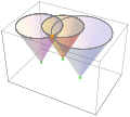
Essentially, the solution, $\scriptstyle (\hat{\boldsymbol{r}}_{\text{rec}},\, \hat{t}_{\text{rec}})$ , is the intersection of light cones.
The posterior distribution of the solution is derived from the product of the distribution of propagating spherical surfaces. (See animation.)

The GPS case

For Global Positioning System (GPS),^[2] the non-closed-form equations in step 3 result in

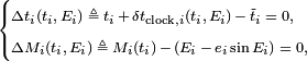
\scriptstyle \begin{cases} \scriptstyle \Delta t_i (t_i,\, E_i) \;\triangleq\; t_i \,+\, \delta t_{\text{clock},i} (t_i,\, E_i) \,-\, \tilde{t}_i \;=\; 0, \\ \scriptstyle \Delta M_i (t_i,\, E_i) \;\triangleq\; M_i (t_i) \,-\, (E_i \,-\, e_i \sin E_i) \;=\; 0, \end{cases}

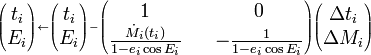
in which $\scriptstyle E_i$ is the orbital eccentric anomaly of satellite $i$ , $\scriptstyle M_i$ is the mean anomaly, $\scriptstyle e_i$ is the eccentricity, and $\scriptstyle \delta t_{\text{clock},i} (t_i,\, E_i) \;=\; \delta t_{\text{clock,sv},i} (t_i) \,+\, \delta t_{\text{orbit-relativ},i} (E_i)$ .

The above can be solved by using the bivariate Newton-Raphson method on $\scriptstyle t_i$ and $\scriptstyle E_i$ . Two times of iteration will be necessary and sufficient in most cases. Its iterative update will be described by using the approximated inverse of Jacobian matrix as follows:

$\scriptscriptstyle \begin{pmatrix} t_i \\ E_i \\ \end{pmatrix} \leftarrow \begin{pmatrix} t_i \\ E_i \\ \end{pmatrix} - \begin{pmatrix} 1 && 0 \\ \frac{\dot{M}_i (t_i)}{1 - e_i \cos E_i} && -\frac{1}{1 - e_i \cos E_i} \\ \end{pmatrix} \begin{pmatrix} \Delta t_i \\ \Delta M_i \\ \end{pmatrix}$

Tropospheric delay should not be ignored, while the Global Positioning System (GPS) specification ^[2] doesn't provide its detailed description.

The GLONASS case

The GLONASS ephemerides don't provide clock biases $\scriptstyle\delta t_{\text{clock,sv},i} (t)$ , but $\scriptstyle\delta t_{\text{clock},i} (t)$ .

Note

In the field of GNSS, $\scriptstyle \tilde{r}_i \;=\; -c (\tilde{t}_i \,-\, \tilde{t}_{\text{rec}})$ is called pseudorange, where $\scriptstyle \tilde{t}_{\text{rec}}$ is a provisional reception time of the receiver. $\scriptstyle \delta t_{\text{clock,rec}} \;=\; \tilde{t}_{\text{rec}} \,-\, t_{\text{rec}}$ is called receiver's clock bias (i.e., clock advance).^[1]
Standard GNSS receivers output $\scriptstyle \tilde{r}_i$ and $\scriptstyle \tilde{t}_{\text{rec}}$ per an observation epoch.
The temporal variation in the relativistic clock bias of satellite is linear if its orbit is circular (and thus its velocity is uniform in inertial frame).
The signal transit time is expressed as $\scriptstyle -(t_i - t_{\text{rec}}) \;=\; \tilde{r}_i/c \,+\, \delta t_{\text{clock},i} \,-\, \delta t_{\text{clock,rec}}$ , whose right side is round-off-error resistive during calculation.
The geometric range is calculated as $\scriptstyle r(\boldsymbol{r}_i,\, \boldsymbol{r}_{\text{rec}}) \;=\; | \Omega_{\text{E}} (t_i \,-\, t_{\text{rec}}) \boldsymbol{r}_{i,\text{ECEF}} \,-\, \boldsymbol{r}_{\text{rec,ECEF}} |$ , where the Earth-centred Earth-fixed (ECEF) rotating frame (e.g., WGS84 or ITRF) is used in the right side and $\scriptstyle \Omega_{\text{E}}$ is the Earth rotating matrix with the argument of the signal transit time.^[2] The matrix can be factorized as $\scriptstyle \Omega_{\text{E}} (t_i \,-\, t_{\text{rec}}) \;=\; \Omega_{\text{E}} (\delta t_{\text{clock,rec}}) \Omega_{\text{E}} (-\tilde{r}_i/c \,-\, \delta t_{\text{clock},i})$ .
The line-of-sight unit vector of satellite observed at $\scriptstyle \boldsymbol{r}_{\text{rec,ECEF}}$ is described as: $\scriptstyle \boldsymbol{e}_{i, \text{rec,ECEF}} \;=\; -\frac{\partial r(\boldsymbol{r}_i,\, \boldsymbol{r}_{\text{rec}})}{\partial \boldsymbol{r}_{\text{rec,ECEF}}}$ .
The satellite-navigation positioning equation may be expressed by using the variables $\scriptstyle \boldsymbol{r}_{\text{rec,ECEF}}$ and $\scriptstyle \delta t_{\text{clock,rec}}$ .
The nonlinearity of the vertical dependency of tropospheric delay degrades the convergence efficiency in the Gauss–Newton iterations in step 7.
The above notation is different from that in the Wikipedia articles, 'Position calculation introduction' and 'Position calculation advanced', of Global Positioning System (GPS).

References

↑ 1.0 1.1 Misra, P. and Enge, P., Global Positioning System: Signals, Measurements, and Performance, 2nd, Ganga-Jamuna Press, 2006.
↑ 2.0 2.1 2.2 2.3 2.4 2.5 The interface specification of NAVSTAR GLOBAL POSITIONING SYSTEM