Functional principal component analysis
Functional principal component analysis (FPCA) is a statistical method for investigating the dominant modes of variation of functional data. Using this method, a random function is represented in the eigenbasis, which is an orthonormal basis of the Hilbert space L2 that consists of the eigenfunctions of the autocovariance operator. FPCA represents functional data in the most parsimonious way, in the sense that when using a fixed number of basis functions, the eigenfunction basis explains more variation than any other basis expansion. FPCA can be applied for representing random functions,[1] or functional regression[2] and classification.
Formulation
For a square-integrable stochastic process X(t), t ∈ 𝒯, let
and
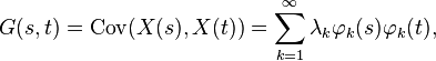
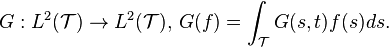
where λ1 ≥ λ2 ≥ ··· ≥ 0 are the eigenvalues and φ1, φ2, ... are the orthonormal eigenfunctions of the linear Hilbert–Schmidt operator
By the Karhunen–Loève theorem, one can express the centered process in the eigenbasis,
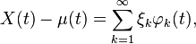
where

is the principal component associated with the k-th eigenfunction φk, with the properties

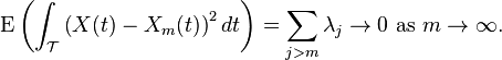
The centered process is then equivalent to ξ1, ξ2, .... A common assumption is that X can be represented by only the first few eigenfunctions (after subtracting the mean function), i.e.
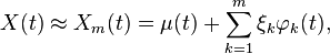
where
Interpretation of eigenfunctions
The first eigenfunction φ1 depicts the dominant mode of variation of X.
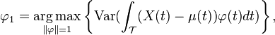
where
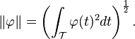
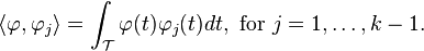
The k-th eigenfunction φk is the dominant mode of variation orthogonal to φ1, φ2, ... , φk-1,

where
Estimation
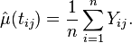
Let Yij = Xi(tij) + εij be the observations made at locations (usually time points) tij, where Xi is the i-th realization of the smooth stochastic process that generates the data, and εij are identically and independently distributed normal random variable with mean 0 and variance σ2, j = 1, 2, ..., mi. To obtain an estimate of the mean function μ(tij), if a dense sample on a regular grid is available, one may take the average at each location tij:
If the observations are sparse, one needs to smooth the data pooled from all observations to obtain the mean estimate,[3] using smoothing methods like local linear smoothing or spline smoothing.
Then the estimate of the covariance function  is obtained by averaging (in the dense case) or smoothing (in the sparse case) the raw covariances

Note that the diagonal elements of Gi should be removed because they contain measurement error.[4]
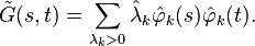
In practice, is discretized to an equal-spaced dense grid, and the estimation of eigenvalues λk and eigenvectors vk is carried out by numerical linear algebra.[5] The eigenfunction estimates  can then be obtained by interpolating the eigenvectors
The fitted covariance should be positive definite and symmetric and is then obtained as
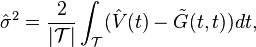
Let  be a smoothed version of the diagonal elements Gi(tij, tij) of the raw covariance matrices. Then is an estimate of (G(t, t) + σ2). An estimate of σ2 is obtained by
 if
if  otherwise
If the observations Xij, j=1, 2, ..., mi are dense in 𝒯, then the k-th FPC ξk can be estimated by numerical integration, implementing

However, if the observations are sparse, this method will not work. Instead, one can use best linear unbiased predictors,[3] yielding
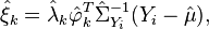
where
 ,
,
and  is evaluated at the grid points generated by tij, j = 1, 2, ..., mi. The algorithm, PACE, has an available Matlab package.[6]
Asymptotic convergence properties of these estimates have been investigated.[3][7][8]
Applications
FPCA can be applied for displaying the modes of functional variation,[1] in scatterplots of FPCs against each other or of responses against FPCs, for modeling sparse longitudinal data,[3] or for functional regression and classification, e.g., functional linear regression.[2] Scree plots and other methods can be used to determine the number of included components.
Connection with principal component analysis
The following table shows a comparison of various elements of principal component analysis (PCA) and FPCA. The two methods are both used for dimensionality reduction. In implementations, FPCA uses a PCA step.
However, PCA and FPCA differ in some critical aspects. First, the order of multivariate data in PCA can be permuted, which has no effect on the analysis, but the order of functional data carries time or space information and cannot be reordered. Second, the spacing of observations in FPCA matters, while there is no spacing issue in PCA. Third, regular PCA does not work for high-dimensional data without regularization, while FPCA has a built-in regularization due to the smoothness of the functional data and the truncation to a finite number of included components.
| Element | In PCA | In FPCA |
|---|---|---|
| Data |  |
 |
| Dimension |  |
 |
| Mean |  |
 |
| Covariance |  |
 |
| Eigenvalues |  |
 |
| Eigenvectors/Eigenfunctions |  |
 |
| Inner Product |  |
 |
| Principal Components |  |
 |
See also
Notes
- ↑ 1.0 1.1 Jones, M. C.; Rice, J. A. (1992). "Displaying the Important Features of Large Collections of Similar Curves". The American Statistician 46 (2): 140. doi:10.1080/00031305.1992.10475870.
- ↑ 2.0 2.1 Yao, F.; Müller, H. G.; Wang, J. L. (2005). "Functional linear regression analysis for longitudinal data". The Annals of Statistics 33 (6): 2873. doi:10.1214/009053605000000660.
- ↑ 3.0 3.1 3.2 3.3 Yao, F.; Müller, H. G.; Wang, J. L. (2005). "Functional Data Analysis for Sparse Longitudinal Data". Journal of the American Statistical Association 100 (470): 577. doi:10.1198/016214504000001745.
- ↑ Staniswalis, J. G.; Lee, J. J. (1998). "Nonparametric Regression Analysis of Longitudinal Data". Journal of the American Statistical Association 93 (444): 1403. doi:10.1080/01621459.1998.10473801.
- ↑ Rice, John; Silverman, B. (1991). "Estimating the Mean and Covariance Structure Nonparametrically When the Data are Curves". Journal of the Royal Statistical Society. Series B (Methodological) (Wiley) 53 (1): 233–243.
- ↑ "PACE: Principal Analysis by Conditional Expectation".
- ↑ Hall, P.; Müller, H. G.; Wang, J. L. (2006). "Properties of principal component methods for functional and longitudinal data analysis". The Annals of Statistics 34 (3): 1493. doi:10.1214/009053606000000272.
- ↑ Li, Y.; Hsing, T. (2010). "Uniform convergence rates for nonparametric regression and principal component analysis in functional/longitudinal data". The Annals of Statistics 38 (6): 3321. doi:10.1214/10-AOS813.
References
- James O. Ramsay; B. W. Silverman (8 June 2005). Functional Data Analysis. Springer. ISBN 978-0-387-40080-8.