Freivalds' algorithm
Freivalds' algorithm (named after Rusins Freivalds) is a probabilistic randomized algorithm used to verify matrix multiplication. Given three n × n matrices A, B, and C, a general problem is to verify whether A × B = C. A naïve algorithm would compute the product A × B explicitly and compare term by term whether this product equals C. However, the best known matrix multiplication algorithm runs in O(n2.3729) time.[1] Freivalds' algorithm utilizes randomization in order to reduce this time bound to O(n2)
[2]
with high probability. In O(kn2) time the algorithm can verify a matrix product with probability of failure less than  .
.
The algorithm
Input
Three n × n matrices A, B, C.
Output
Yes, if A × B = C; No, otherwise.
Procedure
- Generate an n × 1 random 0/1 vector
 .
. - Compute
 .
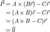
. - Output "Yes" if
 ; "No," otherwise.
Error
If A × B = C, then the algorithm always returns "Yes". If A × B ≠ C, then the probability that the algorithm returns "Yes" is less than or equal to one half. This is called one-sided error.
By iterating the algorithm k times and returning "Yes" only if all iterations yield "Yes", a runtime of O(kn2) and error probability of ≤ 1/2k is achieved.
Example
Suppose one wished to determine whether:
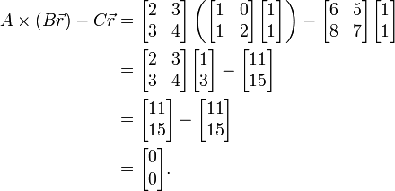
A random two-element vector with entries equal to 0 or 1 is selected — say  — and used to compute:
This yields the zero vector, suggesting the possibility that AB = C. However, if in a second trial the vector  is selected, the result becomes:
The result is nonzero, proving that in fact AB ≠ C.
There are four two-element 0/1 vectors, and half of them give the zero vector in this case ( and
and  ), so the chance of randomly selecting these in two trials (and falsely concluding that AB=C) is 1/22 or 1/4. In the general case, the proportion of r yielding the zero vector may be less than 1/2, and a larger number of trials (such as 20) would be used, rendering the probability of error very small.
Error analysis
Let p equal the probability of error. We claim that if A × B = C, then p = 0, and if A × B ≠ C, then p ≤ 1/2.
Case A × B = C
This is regardless of the value of  , since it uses only that
  . Hence the probability for error in this case is:
Case A × B ≠ C
Let
Where
 .
.
Since  , we have that some element of
  is nonzero. Suppose that the element
  . By the definition of matrix multiplication, we have:
 .
.
For some constant  .
Using Bayes' Theorem, we can partition over
  :
:
-
![\Pr[p_i = 0] = \Pr[p_i = 0 | y = 0]\cdot \Pr[y = 0]\, +\, \Pr[p_i = 0 | y \neq 0] \cdot \Pr[y \neq 0]](../I/m/455a6a17ce499275c733ec200146291a.png)
(1)
We use that:
Plugging these in the equation (1), we get:
Therefore,
This completes the proof.
Ramifications
Simple algorithmic analysis shows that the running time of this algorithm is O(n2), beating the classical deterministic algorithm's bound of O(n3). The error analysis also shows that if we run our algorithm k times, we can achieve an error bound of less than  , an exponentially small quantity. The algorithm is also fast in practice due to wide availability of fast implementations for matrix-vector products. Therefore, utilization of randomized algorithms can speed up a very slow deterministic algorithm. In fact, the best known deterministic matrix multiplication verification algorithm known at the current time is a variant of the Coppersmith–Winograd algorithm with an asymptotic running time of O(n2.3729).[1]
Freivalds' algorithm frequently arises in introductions to probabilistic algorithms due to its simplicity and how it illustrates the superiority of probabilistic algorithms in practice for some problems.
See also
References
- ↑ 1.0 1.1 Virginia Vassilevska Williams. "Breaking the Coppersmith-Winograd barrier".
- ↑ Raghavan, Prabhakar (1997). "Randomized algorithms". ACM Computing Surveys (CSUR) 28. doi:10.1145/234313.234327. Retrieved 2008-12-16.
- Freivalds, R. (1977), “Probabilistic Machines Can Use Less Running Time”, IFIP Congress 1977, pp. 839–842.
| ||||||||||||||||||


![\Pr[\vec{P} \neq 0] = 0](../I/m/cb9829cdf609d403227aaaf2923052fa.png)

![\Pr[p_i = 0 | y = 0] = \Pr[r_j = 0] = \frac{1}{2}](../I/m/80cbfb2617538f5bc113d0c92b535bc8.png)
![\Pr[p_i = 0 | y \neq 0] = \Pr[r_j = 1 \and d_{ij}=-y] \leq \Pr[r_j = 1] = \frac{1}{2}](../I/m/b461802074a1f0ad29738f12e717daac.png)
![\begin{align}
\Pr[p_i = 0] &\leq \frac{1}{2}\cdot \Pr[y = 0] + \frac{1}{2}\cdot \Pr[y \neq 0]\\
&= \frac{1}{2}\cdot \Pr[y = 0] + \frac{1}{2}\cdot (1 - \Pr[y = 0])\\
&= \frac{1}{2}
\end{align}](../I/m/be5fdcceca12522ceee8b2e334fa3885.png)
![\Pr[\vec{P} = 0] = \Pr[p_0 = 0 \and p_1 = 0 \and \dots] \leq \Pr[p_i = 0] \leq \frac{1}{2}.](../I/m/19f8a3f9cca906b028282b34e59592cb.png)