Feedback linearization

Block diagram illustrating the feedback linearization of a nonlinear system

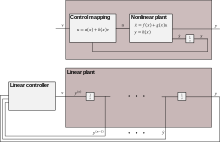
Feedback linearization is a common approach used in controlling nonlinear systems. The approach involves coming up with a transformation of the nonlinear system into an equivalent linear system through a change of variables and a suitable control input. Feedback linearization may be applied to nonlinear systems of the form

\begin{align}\dot{x} &= f(x) + g(x)u \qquad &(1)\\ y &= h(x) \qquad \qquad \qquad &(2)\end{align}

where $x \in \mathbb{R}^n$ is the state vector, $u \in \mathbb{R}^p$ is the vector of inputs, and $y \in \mathbb{R}^m$ is the vector of outputs. The goal is to develop a control input

u = a(x) + b(x)v\,

that renders a linear input–output map between the new input $v$ and the output. An outer-loop control strategy for the resulting linear control system can then be applied.

Feedback Linearization of SISO Systems

Here, we consider the case of feedback linearization of a single-input single-output (SISO) system. Similar results can be extended to multiple-input multiple-output (MIMO) systems. In this case, $u \in \mathbb{R}$ and $y \in \mathbb{R}$ . We wish to find a coordinate transformation $z = T(x)$ that transforms our system (1) into the so-called normal form which will reveal a feedback law of the form

u = a(x) + b(x)v\,

that will render a linear input–output map from the new input $v \in \mathbb{R}$ to the output $y$ . To ensure that the transformed system is an equivalent representation of the original system, the transformation must be a diffeomorphism. That is, the transformation must not only be invertible (i.e., bijective), but both the transformation and its inverse must be smooth so that differentiability in the original coordinate system is preserved in the new coordinate system. In practice, the transformation can be only locally diffeomorphic, but the linearization results only hold in this smaller region.

We require several tools before we can solve this problem.

Lie derivative

The goal of feedback linearization is to produce a transformed system whose states are the output $y$ and its first $(n-1)$ derivatives. To understand the structure of this target system, we use the Lie derivative. Consider the time derivative of (2), which we can compute using the chain rule,

\begin{align} \dot{y} = \frac{\operatorname{d}h(x)}{\operatorname{d}t} &=\frac{\operatorname{d}h(x)}{\operatorname{d}x}\dot{x}\\ &= \frac{\operatorname{d}h(x)}{\operatorname{d}x}f(x) + \frac{\operatorname{d}h(x)}{\operatorname{d}x}g(x)u \end{align}

Now we can define the Lie derivative of $h(x)$ along $f(x)$ as,

L_{f}h(x) = \frac{\operatorname{d}h(x)}{\operatorname{d}x}f(x),

and similarly, the Lie derivative of $h(x)$ along $g(x)$ as,

L_{g}h(x) = \frac{\operatorname{d}h(x)}{\operatorname{d}x}g(x).

With this new notation, we may express $\dot{y}$ as,

\dot{y} = L_{f}h(x) + L_{g}h(x)u

Note that the notation of Lie derivatives is convenient when we take multiple derivatives with respect to either the same vector field, or a different one. For example,

L_{f}^{2}h(x) = L_{f}L_{f}h(x) = \frac{\operatorname{d}(L_{f}h(x))}{\operatorname{d}x}f(x),

and

L_{g}L_{f}h(x) = \frac{\operatorname{d}(L_{f}h(x))}{\operatorname{d}x}g(x).

Relative degree

In our feedback linearized system made up of a state vector of the output $y$ and its first $(n-1)$ derivatives, we must understand how the input $u$ enters the system. To do this, we introduce the notion of relative degree. Our system given by (1) and (2) is said to have relative degree $r \in \mathbb{W}$ at a point $x_0$ if,

L_{g}L_{f}^{k}h(x) = 0 \qquad \forall x

in a neighbourhood of

x_0

and all

k \leq r-2

L_{g}L_{f}^{r-1}h(x_0) \neq 0

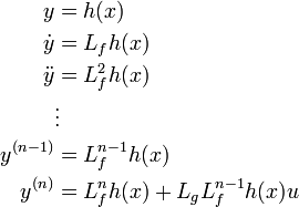
Considering this definition of relative degree in light of the expression of the time derivative of the output $y$ , we can consider the relative degree of our system (1) and (2) to be the number of times we have to differentiate the output $y$ before the input $u$ appears explicitly. In an LTI system, the relative degree is the difference between the degree of the transfer function's denominator polynomial (i.e., number of poles) and the degree of its numerator polynomial (i.e., number of zeros).

Linearization by feedback

For the discussion that follows, we will assume that the relative degree of the system is $n$ . In this case, after differentiating the output $n$ times we have,

\begin{align} y &= h(x)\\ \dot{y} &= L_{f}h(x)\\ \ddot{y} &= L_{f}^{2}h(x)\\ &\vdots\\ y^{(n-1)} &= L_{f}^{n-1}h(x)\\ y^{(n)} &= L_{f}^{n}h(x) + L_{g}L_{f}^{n-1}h(x)u \end{align}

where the notation $y^{(n)}$ indicates the $n$ th derivative of $y$ . Because we assumed the relative degree of the system is $n$ , the Lie derivatives of the form $L_{g}L_{f}^{i}h(x)$ for $i = 1, \dots, n-2$ are all zero. That is, the input $u$ has no direct contribution to any of the first $(n-1)$ th derivatives.

The coordinate transformation $T(x)$ that puts the system into normal form comes from the first $(n-1)$ derivatives. In particular,

z = T(x) = \begin{bmatrix}z_1(x) \\ z_2(x) \\ \vdots \\ z_n(x) \end{bmatrix} = \begin{bmatrix}y\\ \dot{y}\\ \vdots\\ y^{(n-1)} \end{bmatrix} = \begin{bmatrix}h(x) \\ L_{f}h(x) \\ \vdots \\ L_{f}^{n-1}h(x) \end{bmatrix}

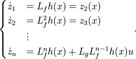
transforms trajectories from the original $x$ coordinate system into the new $z$ coordinate system. So long as this transformation is a diffeomorphism, smooth trajectories in the original coordinate system will have unique counterparts in the $z$ coordinate system that are also smooth. Those $z$ trajectories will be described by the new system,

\begin{cases}\dot{z}_1 &= L_{f}h(x) = z_2(x)\\ \dot{z}_2 &= L_{f}^{2}h(x) = z_3(x)\\ &\vdots\\ \dot{z}_n &= L_{f}^{n}h(x) + L_{g}L_{f}^{n-1}h(x)u\end{cases}.

Hence, the feedback control law

u = \frac{1}{L_{g}L_{f}^{n-1}h(x)}(-L_{f}^{n}h(x) + v)

renders a linear input–output map from $v$ to $z_1 = y$ . The resulting linearized system

\begin{cases}\dot{z}_1 &= z_2\\ \dot{z}_2 &= z_3\\ &\vdots\\ \dot{z}_n &= v\end{cases}

is a cascade of $n$ integrators, and an outer-loop control $v$ may be chosen using standard linear system methodology. In particular, a state-feedback control law of

v = -Kz\qquad,

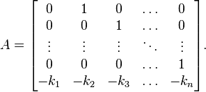
where the state vector $z$ is the output $y$ and its first $(n-1)$ derivatives, results in the LTI system

\dot{z} = Az

with,

A = \begin{bmatrix} 0 & 1 & 0 & \ldots & 0 \\ 0 & 0 & 1 & \ldots & 0 \\ \vdots & \vdots & \vdots & \ddots & \vdots \\ 0 & 0 & 0 & \ldots & 1 \\ -k_1 & -k_2 & -k_3 & \ldots & -k_n \end{bmatrix}.

So, with the appropriate choice of $k$ , we can arbitrarily place the closed-loop poles of the linearized system.

Unstable zero dynamics

Feedback linearization can be accomplished with systems that have relative degree less than $n$ . However, the normal form of the system will include zero dynamics (i.e., states that are not observable from the output of the system) that may be unstable. In practice, unstable dynamics may have deleterious effects on the system (e.g., it may be dangerous for internal states of the system to grow unbounded). These unobservable states may be controllable or at least stable, and so measures can be taken to ensure these states do not cause problems in practice.

External links

ECE 758: Modeling and Nonlinear Control of a Single-link Flexible Joint Manipulator – Gives explanation and an application of feedback linearization.
ECE 758: Ball-in-Tube Linearization Example – Trivial application of linearization for a system already in normal form (i.e., no coordinate transformation necessary).
Wolfram language functions to do feedback linearization, compute relative orders, and determine zero dynamics.