Feasible region
In mathematical optimization, a feasible region, feasible set, search space, or solution space is the set of all possible points (sets of values of the choice variables) of an optimization problem that satisfy the problem's constraints, potentially including inequalities, equalities, and integer constraints. This is the initial set of candidate solutions to the problem, before the set of candidates has been narrowed down.
For example, consider the problem
- Minimize

with respect to the variables  and
and 
subject to

and

Here the feasible set is the set of pairs (x1, x2) in which the value of x1 is at least 1 and at most 10 and the value of x2 is at least 5 and at most 12. Note that the feasible set of the problem is separate from the objective function, which states the criterion to be optimized and which in the above example is 
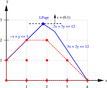
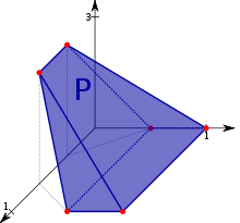
In many problems, the feasible set reflects a constraint that one or more variables must be non-negative. In pure integer programming problems, the feasible set is the set of integers (or some subset thereof). In linear programming problems, the feasible set is a convex polytope: a region in multidimensional space whose boundaries are formed by hyperplanes and whose corners are vertices.
Constraint satisfaction is the process of finding a point in the feasible region.
Convex feasible set

A convex feasible set is one in which a line segment connecting any two feasible points goes through only other feasible points, and not through any points outside the feasible set. Convex feasible sets arise in many types of problems, including linear programming problems, and they are of particular interest because, if the problem has a convex objective function that is to be maximized, it will generally be easier to solve in the presence of a convex feasible set and any local optimum will also be a global optimum.
No feasible set
If the constraints of an optimization problem are mutually contradictory, there are no points that satisfy all the constraints and thus the feasible region is the null set. In this case the problem has no solution and is said to be infeasible.
Bounded and unbounded feasible sets

Feasible sets may be bounded or unbounded. For example, the feasible set defined by the constraint set {x ≥ 0, y ≥ 0} is unbounded because in some directions there is no limit on how far one can go and still be in the feasible region. In contrast, the feasible set formed by the constraint set {x ≥ 0, y ≥ 0, x + 2y ≤ 4} is bounded because the extent of movement in any direction is limited by the constraints.
In linear programming problems with n variables, a necessary but not sufficient condition for the feasible set to be bounded is that the number of constraints be at least n + 1 (as illustrated by the above example).
If the feasible set is unbounded, there may or may not be an optimum, depending on the specifics of the objective function. For example, if the feasible region is defined by the constraint set {x ≥ 0, y ≥ 0}, then the problem of maximizing x + y has no optimum since any candidate solution can be improved upon by increasing x or y; yet if the problem is to minimize x + y, then there is an optimum (specifically at (x, y) = (0, 0)).