Euler equations (fluid dynamics)
In fluid dynamics, the Euler equations are a set of quasilinear hyperbolic equations governing adiabatic and inviscid flow. They are named after Leonhard Euler. The equations represent Cauchy equations of conservation of mass (continuity), and balance of momentum and energy, and can be seen as particular Navier–Stokes equations with zero viscosity and zero thermal conductivity.[1] The Euler equations can be applied to incompressible and to compressible flow– assuming that the divergence of the flow velocity field is zero, or using either as an additional constraint an appropriate equation of state respectively. Historically, only the incompressible equations have been derived by Euler. However, fluid dynamics literature often refers to the full set – including the energy equation – together as "the Euler equations".[2]
Without external field (in the limit of high Froude number) Euler equations are conservation equations. Like any Cauchy equation, the Euler equations are usually written in one of two forms: the "conservation form" and the "lagrangian form". The conservation form emphasizes the physical interpretation of the equations as (quasi-)conservation laws through a control volume fixed in space, and is the most important for these equations also from a numerical point of view. The lagrangian form emphasizes changes to the state in a frame of reference moving with the fluid.
History
The Euler equations first appeared in published form in Euler's article "Principes généraux du mouvement des fluides", published in Mémoires de l'Academie des Sciences de Berlin in 1757 (in this article Euler actually published only the general form of the continuity equation and the momentum equation;[3] the energy balance equation would be obtained a century later). They were among the first partial differential equations to be written down. At the time Euler published his work, the system of equations consisted of the momentum and continuity equations, and thus was underdetermined except in the case of an incompressible fluid. An additional equation, which was later to be called the adiabatic condition, was supplied by Pierre-Simon Laplace in 1816.
During the second half of the 19th century, it was found that the equation related to the balance of energy must at all times be kept, while the adiabatic condition is a consequence of the fundamental laws in the case of smooth solutions. With the discovery of the special theory of relativity, the concepts of energy density, momentum density, and stress were unified into the concept of the stress–energy tensor, and energy and momentum were likewise unified into a single concept, the energy–momentum vector.[4]
Incompressible Euler equations with constant and uniform density
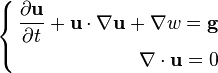
In convective form (i.e. the form with the convective operator made explicit in the momentum equation), the incompressible Euler equations in case of density constant in time and uniform in space are:[5]
Incompressible Euler equations with constant and uniform density (convective form)
where:
- u is the flow velocity vector, with components in a N-dimensional space u1, u2 ... uN,
 denotes the scalar product,
- ∇ is the nabla operator, here used in the flow velocity divergence (first equation), and in flow velocity and specific pressure gradients (second equation), and
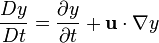
 is the convective operator,
- w is the specific (with the sense of per unit mass) thermodynamic work, the internal source term.
-
 represents body accelerations (per unit mass) acting on the continuum, for example gravity, inertial accelerations, electric field acceleration, and so on.
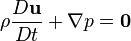
The first equation is the Euler momentum equation with uniform density (for this equation it could also not be constant in time): in fact for a flow with uniform density ρ0 the following identity holds:
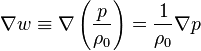
where p is the mechanic pressure. The second equation is the incompressible constraint (the choice of the order of presentation is not casual, but underlines the fact that the incompressible constraint does never come from the continuity equation, but is a further constraint to the original balance equations. Notably, the continuity equation would be required also in this incompressible case as an additional third equation in case of density varying in time or varying in space. For example with density uniform but varying in time, the continuity equation to be added to the above set would correspond to:

So the case of constant and uniform density is the only one not requiring the continuity equation as additional equation regardless of the presence or absence of the incompressible contraint. In fact, the case of incompressible Euler equations with constant and uniform density being analised is a toy model very simple as featuring only two simplified equations, so it is ideal for didactical purposes even if with limited physical relevancy.
The equations above thus represent respectively conservation of mass (1 scalar equation) and momentum (1 vector equation containing N scalar components, where N is the physical dimension of the space of interest). In 3D for example N=3 and the r and u vectors are explicitly ( x1, x2, x3 ) and ( u1, u2, u3 ). Flow velocity and pressure are the so-called physical variables.[1]
These equations may be expressed in subscript notation:
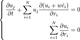
where the i and j subscripts label the N-dimensional space components. These equations may be more succinctly expressed using Einstein notation:
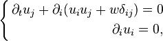
where the i and j subscripts label the N-dimensional space components, and δ is the Kroenecker delta. In 3D N=3 and the r and u vectors are explicitly ( x1, x2, x3 ) and ( u1, u2, u3 ), and matched indices imply a sum over those indices and  and
and  .
.
Nondimensionalisation
In order to make the equations dimensionless, a characteristic length r0, and a characteristic velocity u0, need to be defined. These should be chosen such that the dimensionless variables are all of order one. The following dimensionless variables are thus obtained:


and of the field unit vector:

Substitution of these inversed relations in Euler equations, defining the Froude number, yields (omitting the * at apix):
Incompressible Euler equations with constant and uniform density (nondimensional form)
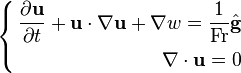
Euler equations in the Froude limit (no external field) are named free equations and are conservative. The limit of high Froude numbers (low external field) is thus notable and can be studied with perturbation theory.
Conservation form
The conservation form emphasizes the physical origins of Euler equations, and especially the contracted form is often the most convenient one for computational fluid dynamics simulations. Computationally, there are some advantages in using the conserved variables. This gives rise to a large class of numerical methods called conservative methods.[1]
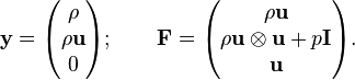
The free Euler equations are conservative, in the sense they are equivalent to a conservation equation:
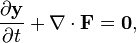
or simply in Einstein notation:
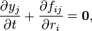
where the conservation quantity y in this case is a vector, and F is a flux matrix. This is now being proved.
First, the following identities hold:

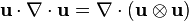
where  denotes the tensor product. The same identited expressed in Einstein notation are:

where I is the identity matrix with dimension N and δij its general element, the Kroenecker delta.
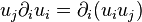
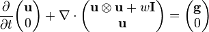
Thanks to these vector identities, the incompressible Euler equations with constant and uniform density and without external field can be put in the so-called conservation (or Eulerian) differential form, with vector notation:
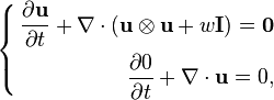
or with Einstein notation:
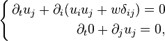
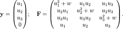
Then incompressible Euler equations with uniform density have conservation variables:
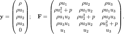
Note that in the second component u is by itself a vector, with length N, so y has length N+1 and F has size N(N+1). In 3D for example y has length 4, I has size 3x3 and F has size 3x4, so the explicit forms are:
Finally Euler equations can be recast into the particular equation:
Incompressible Euler equation(s) with constant and uniform density (conservation form)
Spatial dimensions
For certain problems, especially when used to analyze compressible flow in a duct or in case the flow is cylindrically or spherically symmetric, the one-dimensional Euler equations are a useful first approximation. Generally, the Euler equations are solved by Riemann's method of characteristics. This involves finding curves in plane of independent variables (i.e., x and t) along which partial differential equations (PDE's) degenerate into ordinary differential equations (ODE's). Numerical solutions of the Euler equations rely heavily on the method of characteristics.
Incompressible Euler equations
In convective form the incompressible Euler equations in case of density variable in space are:[5]
Incompressible Euler equations (convective form)
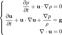
where the additional variables are:
- ρ is the fluid mass density,
- p is the pressure,
 .
.
The first equation, which is the new one, is the incompressible continuity equation. In fact the continuity equation:
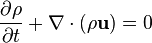
by the Leibnitz rule can be explicited as:
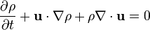
The last term is identically zero for the incompressibility constraint.
Conservation form
The incompressible Euler equations in the Froude limit are equivalent to a single conservation equation with conserved quantity and associated flux respectively:
Here y has length N+2 and F has size N(N+2). In 3D for example y has length 5, I has size 3x3 and F has size 3x5, so the explicit forms are:
In general (not only in the Froude limit) Euler equations are expressible as:
Incompressible Euler equation(s) (conservation form)
Euler equations
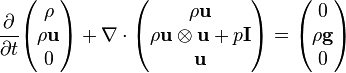
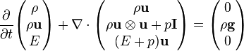
In differential form, the compressible (and most general) Euler equations are:
Euler equations (convective form)
![\left\{\begin{align}
{\partial\rho\over\partial t}+
\nabla\cdot(\rho\bold u)=0\\[1.2ex]
\rho\frac{\partial \mathbf{ u}}{\partial t} + \rho\mathbf{u} \cdot \nabla \mathbf{u} + \nabla p = \rho \mathbf{g} \\[1.2ex]
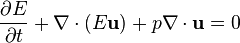
{\partial E\over\partial t}+
\nabla\cdot(\bold u(E+p))=0,
\end{align}\right.](../I/m/17d55252b9b8c921db151a9efe07858a.png)
where the additional variables are:
- ρu is the momentum density vector,
- E = ρ e + ½ ρ u2 is the total energy density (total energy per unit volume), with e being the specific internal energy (internal energy per unit mass),
The equations above thus represent conservation of mass, momentum, and energy. Mass density, Flow velocity and pressure are the so-called physical variables, while mass density, momentum density and total energy density are the so-called conserved variables.[1] These equations may be expressed in subscript notation. The momentum equation (the second one) includes the divergence of a dyadic product.
Conservation form
The Euler equations in the Froude limit are equivalent to a single conservation equation with conserved quantity and associated flux respectively:
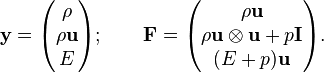
Here y has length N+2 and F has size N(N+2). In 3D for example y has length 5, I has size 3x3 and F has size 3x5, so the explicit forms are:
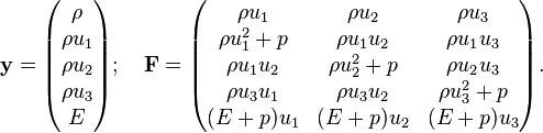
In general (not only in the Froude limit) Euler equations are expressible as:
Euler equation(s) (conservation form)
Jacobian form and sound equations
Expanding the fluxes can be an important part of constructing numerical solvers, for example by exploiting (approximate) solutions to the Riemann problem. From the original equations as given above in vector form, the equations are written as:
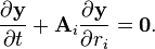
where Ai are called the flux Jacobians defined as the matrices:
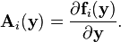
Here, the flux Jacobians Ai are still functions of the state vector y, so this form of the Euler equations is quasilinear, just like the original equations. This Jacobian form is equivalent to the vector equation, at least in regions where the state vector y varies smoothly.
The compressible Euler equations can be decoupled into a set of N+2 wave equations that describes sound in Eulerian continuum if they are expressed in characteristic variables instead of conserved variables. As an example, the one-dimensional (1-D) Euler equations in Jacobian form is considered:
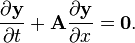
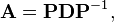
In 1D there is only one matrix A. It is diagonalizable, which means it can be decomposed with a projection matrix into a diagonal matrix:
![\mathbf{P}=[ \mathbf{p}_1, \mathbf{p}_2, \mathbf{p}_3] =\left[
\begin{array}{c c c}
1 & 1 & 1 \\
u-a & u & u+a \\
H-u a & \frac{1}{2} u^2 & H+u a \\
\end{array}
\right],](../I/m/0ef15000e2abfe3752c76eff1a6298cb.png)
Here p1, p2, p3 are the right eigenvectors of the matrix A corresponding with the eigenvalues λ1, λ2 and λ3, and the total enthalpy density is defined as:

Defining the characteristic variables as:

Since A is constant, multiplying the original 1-D equation in flux-Jacobian form with P−1 yields:
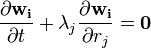
The equations have been decoupled into N+2 wave equations, with the eigenvalues being the wave speeds. The variables wi are called Riemann invariants or, for general hyperbolic systems, they are called characteristic variables.
Sound in ideal gas
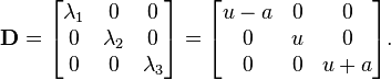
If the equation of state is the ideal gas law, to derive the full Jacobians in matrix form, as given below:[6]
Flux Jacobians in matrix form for an ideal gas in 3D Cartesian frame of reference (x,y,z) The x-direction flux Jacobian: The y-direction flux Jacobian:
The z-direction flux Jacobian:
Where
 .
.
![\bold A_x= \left[
\begin{array}{c c c c c}
0 & 1 & 0 & 0 & 0 \\
\hat{\gamma}H-u^2-a^2 & (3-\gamma)u & -\hat{\gamma}v & -\hat{\gamma}w & \hat{\gamma} \\
-uv & v & u & 0 & 0 \\
-uw & w & 0 & u & 0 \\
u[(\gamma-2)H-a^2] & H-\hat{\gamma}u^2 & -\hat{\gamma}uv & -\hat{\gamma}uw & \gamma u
\end{array}
\right].](../I/m/882943d93513c9140b3419d2c4fda8e3.png)
![\bold A_y= \left[
\begin{array}{c c c c c}
0 & 0 & 1 & 0 & 0 \\
-vu & v & u & 0 & 0 \\
\hat{\gamma}H-v^2-a^2 & -\hat{\gamma}u & (3-\gamma)v & -\hat{\gamma}w & \hat{\gamma} \\
-vw & 0 & w & v & 0 \\
v[(\gamma-2)H-a^2] & -\hat{\gamma}uv & H-\hat{\gamma}v^2 & -\hat{\gamma}vw & \gamma v
\end{array}
\right].](../I/m/ac5e54926ed046904743f5e615ce3c72.png)
![\bold A_z= \left[
\begin{array}{c c c c c}
0 & 0 & 0 & 1 & 0 \\
-uw & w & 0 & u & 0 \\
-vw & 0 & w & v & 0 \\
\hat{\gamma}H-w^2-a^2 & -\hat{\gamma}u & -\hat{\gamma}v & (3-\gamma)w& \hat{\gamma} \\
w[(\gamma-2)H-a^2] & -\hat{\gamma}uw & -\hat{\gamma}vw & H-\hat{\gamma}w^2 & \gamma w
\end{array}
\right].](../I/m/cc20c975b8149c9404f344250f0acb17.png)
The speed of sound a is given by:
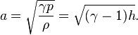
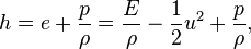
where the enthalpy density h is defined (in general, not only in case of ideal gas) as:
Derivation
Euler equations can be obtained by linearization of some more precise equations like Navier-Stokes equations in around a local equilibrium state given by a Maxwellian y = y0, and are given by:
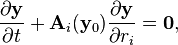
where Ai(y0), are the values of respectively Ai(y) at some reference state y = y0.
Lagrangian form
In differential material or lagrangian form, the equations are:
![\begin{align}
{D\rho\over D t}+ \rho \nabla \cdot \bold u
=0\\[1.2ex]
\frac{D\bold u}{D t}+\frac {\nabla p} \rho=\bold{0}
\\[1.2ex]
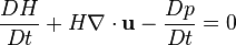
{D H \over D t} +
H \nabla \cdot \bold u - \frac{D p}{D t}=0,
\end{align}](../I/m/edcfea9118442c90e5056476bcbea2d1.png)
Where the time material derivative has been used:
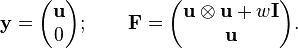
In fact by subtracting the velocity times the mass conservation term, the momentum equation in conservation form, can also be expressed as:
![[\partial_t(\rho u_j)+\partial_i(\rho u_i u_j)+\partial_j p] - u_j[\partial_t \rho+\partial_i(\rho u_i)]=](../I/m/c3cd6a7aba993c4fa2ebf6924acc7add.png)

or, in vector notation:
which is a continuum mechanics form for Newton's second law of motion. Similarly, by subtracting the velocity times the above momentum conservation term, the third equation (energy conservation), can also be expressed as:

or
that can be contracted with the material derivative as:
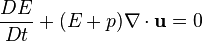
or changing the variable from total energy density to total enthalpy density:
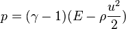
Constraints
In N space dimensions there are thus N+2 equations and N+3 unknowns. Closing the system requires an equation of state; the most commonly used is the ideal gas law:
 where
where
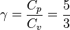 is the adiabatic index of an ideal gas.
Derivation (ideal gas):
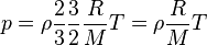
Thermal equation of state is

and caloric equation of state is
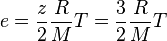 z is number of degrees of freedom (z=3 monoatomic gas).
This leads to
z is number of degrees of freedom (z=3 monoatomic gas).
This leads to
Note the odd form for the energy equation; see Rankine–Hugoniot equation. The extra terms involving p may be interpreted as the mechanical work done on a fluid element by its neighbor fluid elements. These terms sum to zero in an incompressible fluid.
The well-known Bernoulli's equation can be derived by integrating Euler's equation along a streamline, under the assumption of constant density and a sufficiently stiff equation of state.
Steady flow in material coordinates
In the case of steady flow, it is convenient to choose the Frenet–Serret frame along a streamline as the coordinate system for describing the steady momentum Euler equation:[7]
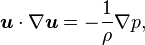
where u, p and ρ denote the flow velocity, the pressure and the density, respectively.
Let {es, en, eb } be a Frenet–Serret orthonormal basis which consists of a tangential unit vector, a normal unit vector, and a binormal unit vector to the streamline, respectively. Since a streamline is a curve that is tangent to the velocity vector of the flow, the left-handed side of the above equation, the convective derivative of velocity, can be described as follows:
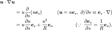
where R is the radius of curvature of the streamline.
Therefore, the momentum part of the Euler equations for a steady flow is found to have a simple form:
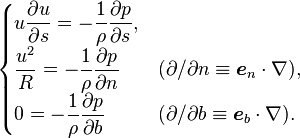
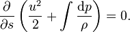
For barotropic flow ( ρ=ρ(p) ), Bernoulli's equation is derived from the first equation:
The second equation expresses that, in the case the streamline is curved, there should exist a pressure gradient normal to the streamline because the centripetal acceleration of the fluid parcel is only generated by the normal pressure gradient.
The third equation expresses that pressure is constant along the binormal axis.
Streamline curvature theorem

Let r be the distance from the center of curvature of the streamline, then the second equation is written as follows:
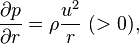
where 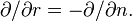
This equation states:
In a steady flow of an inviscid fluid without external forces, the center of curvature of the streamline lies in the direction of decreasing radial pressure.
Although this relationship between the pressure field and flow curvature is very useful, it doesn't have a name in the English-language scientific literature.[8] Japanese fluid-dynamicists call the relationship the "Streamline curvature theorem". [9]
This "theorem" explains clearly why there are such low pressures in the centre of vortices,[8] which consist of concentric circles of streamlines. This also is a way to intuitively explain why airfoils generate lift forces.[8]
Shock waves
The Euler equations are quasilinear hyperbolic equations and their general solutions are waves. Under certain assumptions they can be simplified leading to Burgers equation. Much like the familiar oceanic waves, waves described by the Euler Equations 'break' and so-called shock waves are formed; this is a nonlinear effect and represents the solution becoming multi-valued. Physically this represents a breakdown of the assumptions that led to the formulation of the differential equations, and to extract further information from the equations we must go back to the more fundamental integral form. Then, weak solutions are formulated by working in 'jumps' (discontinuities) into the flow quantities – density, velocity, pressure, entropy – using the Rankine–Hugoniot shock conditions. Physical quantities are rarely discontinuous; in real flows, these discontinuities are smoothed out by viscosity and by heat transfer. (See Navier–Stokes equations)
Shock propagation is studied – among many other fields – in aerodynamics and rocket propulsion, where sufficiently fast flows occur.
See also
- Bernoulli's theorem
- Kelvin's circulation theorem
- Cauchy equations
- Madelung equations
- Froude number
- Navier-Stokes equations
Notes
- ↑ 1.0 1.1 1.2 1.3 see Toro, p. 24
- ↑ Anderson, John D. (1995), Computational Fluid Dynamics, The Basics With Applications. ISBN 0-07-113210-4
- ↑ E226 -- Principes generaux du mouvement des fluides
- ↑ Christodoulou, Demetrios (October 2007). "The Euler Equations of Compressible Fluid Flow" (PDF). Bulletin of the American Mathematical Society 44 (4): 581–602. doi:10.1090/S0273-0979-07-01181-0. Retrieved June 13, 2009.
- ↑ 5.0 5.1 Hunter, J.K. An Introduction to the Incompressible Euler Equations
- ↑ See Toro (1999)
- ↑ James A. Fay (June 1994). Introduction to Fluid Mechanics. MIT Press. ISBN 0-262-06165-1. see "4.5 Euler's Equation in Streamline Coordinates" pp.150-pp.152 (http://books.google.com/books?id=XGVpue4954wC&pg=150)
- ↑ 8.0 8.1 8.2 Babinsky, Holger (November 2003), "How do wings work?" (PDF), Physics Education
- ↑ 今井 功 (IMAI, Isao) (November 1973). 『流体力学(前編)』(Fluid Dynamics 1) (in Japanese). 裳華房 (Shoukabou). ISBN 4-7853-2314-0.
Further reading
- Batchelor, G. K. (1967). An Introduction to Fluid Dynamics. Cambridge University Press. ISBN 0-521-66396-2.
- Thompson, Philip A. (1972). Compressible Fluid Flow. New York: McGraw-Hill. ISBN 0-07-064405-5.
- Toro, E.F. (1999). Riemann Solvers and Numerical Methods for Fluid Dynamics. Springer-Verlag. ISBN 3-540-65966-8.