Error function

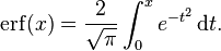
In mathematics, the error function (also called the Gauss error function) is a special function (non-elementary) of sigmoid shape that occurs in probability, statistics, and partial differential equations describing diffusion. It is defined as:[1][2]
The complementary error function, denoted erfc, is defined as
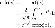
which also defines erfcx, the scaled complementary error function[3] (which can be used instead of erfc to avoid arithmetic underflow[3][4]). Another form of  is known as Craig's formula:[5]
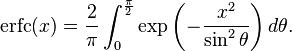
The imaginary error function, denoted erfi, is defined as
 ,
,
where D(x) is the Dawson function (which can be used instead of erfi to avoid arithmetic overflow[3]).
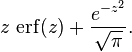
When the error function is evaluated for arbitrary complex arguments z, the resulting complex error function is usually discussed in scaled form as the Faddeeva function:

The name "error function"
The error function is used in measurement theory (using probability and statistics), and although its use in other branches of mathematics has nothing to do with the characterization of measurement errors, the name has stuck.
The error function is related to the cumulative distribution  , the integral of the standard normal distribution, by[2]
The error function, evaluated at  for positive x values, gives the probability that a measurement, under the influence of normally distributed errors with standard deviation
  , has a distance less than x from the mean value.[6] This function is used in statistics to predict behavior of any sample with respect to the population mean. This usage is similar to the Q-function, which in fact can be written in terms of the error function.
Properties


The property  means that the error function is an odd function. This directly results from the fact that the integrand
  is an even function.
For any complex number z:

where  is the complex conjugate of z.
The integrand ƒ = exp(−z2) and ƒ = erf(z) are shown in the complex z-plane in figures 2 and 3. Level of Im(ƒ) = 0 is shown with a thick green line. Negative integer values of Im(ƒ) are shown with thick red lines. Positive integer values of Im(f) are shown with thick blue lines. Intermediate levels of Im(ƒ) = constant are shown with thin green lines. Intermediate levels of Re(ƒ) = constant are shown with thin red lines for negative values and with thin blue lines for positive values.
At the real axis, erf(z) approaches unity at z → +∞ and −1 at z → −∞. At the imaginary axis, it tends to ±i∞.
Taylor series
The error function is an entire function; it has no singularities (except that at infinity) and its Taylor expansion always converges.
The defining integral cannot be evaluated in closed form in terms of elementary functions, but by expanding the integrand e−z2 into its Taylor series and integrating term by term, one obtains the error function's Taylor series as:

which holds for every complex number z. The denominator terms are sequence A007680 in the OEIS.
For iterative calculation of the above series, the following alternative formulation may be useful:
because  expresses the multiplier to turn the kth term into the (k + 1)th term (considering z as the first term).
The error function at +∞ is exactly 1 (see Gaussian integral).
The derivative of the error function follows immediately from its definition:
An antiderivative of the error function is
Higher order derivatives are given by

where  are the probabilists' Hermite polynomials.[7]
Bürmann series
An expansion,[8] which converges more rapidly for all real values of  than a Taylor expansion, is obtained by using Hans Heinrich Bürmann's theorem:[9]
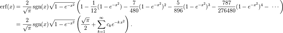
By keeping only the first two coefficients and choosing  and
and  , the resulting approximation shows its largest relative error at
  , where it is less than
  :
:

Inverse functions

The inverse error function can be defined in terms of the Maclaurin series
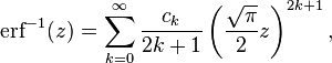
where c0 = 1 and

So we have the series expansion (note that common factors have been canceled from numerators and denominators):

(After cancellation the numerator/denominator fractions are entries A092676/A132467 in the OEIS; without cancellation the numerator terms are given in entry A002067.) Note that the error function's value at ±∞ is equal to ±1.
The inverse complementary error function is defined as

Asymptotic expansion
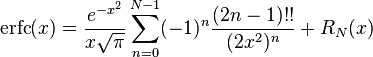
A useful asymptotic expansion of the complementary error function (and therefore also of the error function) for large real x is
![\mathrm{erfc}(x) = \frac{e^{-x^2}}{x\sqrt{\pi}}\left [1+\sum_{n=1}^\infty (-1)^n \frac{1\cdot3\cdot5\cdots(2n-1)}{(2x^2)^n}\right ]=\frac{e^{-x^2}}{x\sqrt{\pi}}\sum_{n=0}^\infty (-1)^n \frac{(2n-1)!!}{(2x^2)^n},\,](../I/m/03fae1c24fcff15dea8fa72bb4675255.png)
where (2n – 1)!! is the double factorial: the product of all odd numbers up to (2n – 1). This series diverges for every finite x, and its meaning as asymptotic expansion is that, for any  one has
where the remainder, in Landau notation, is
 as
as  .
.
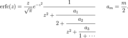
Indeed, the exact value of the remainder is
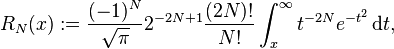
which follows easily by induction, writing 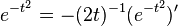 and integrating by parts.
For large enough values of x, only the first few terms of this asymptotic expansion are needed to obtain a good approximation of erfc(x) (while for not too large values of x note that the above Taylor expansion at 0 provides a very fast convergence).
Continued fraction expansion
A continued fraction expansion of the complementary error function is:[10]
Integral of error function with Gaussian density function
![\operatorname{erf} \left[ \frac{b-ac}{\sqrt{1+2 a^2 d^2}} \right] = \int\limits_{-\infty}^{\infty} {\rm d} x \frac{\operatorname{erf} \left(ax+b \right)}{\sqrt{2\pi d^2}} \exp{\left[-\frac{(x+c)^2}{2 d^2} \right]}, \ \ a,b,c,d \in \mathbb{R}](../I/m/3934ca16b3cf19d0bcad6422c4693f83.png)
Approximation with elementary functions
Abramowitz and Stegun give several approximations of varying accuracy (equations 7.1.25–28). This allows one to choose the fastest approximation suitable for a given application. In order of increasing accuracy, they are:
-
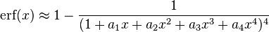 (maximum error: 5×10⁻⁴)
where a1 = 0.278393, a2 = 0.230389, a3 = 0.000972, a4 = 0.078108
-
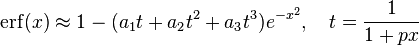 (maximum error: 2.5×10⁻⁵)
where p = 0.47047, a1 = 0.3480242, a2 = −0.0958798, a3 = 0.7478556
-
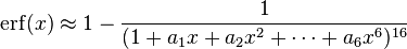 (maximum error: 3×10⁻⁷)
where a1 = 0.0705230784, a2 = 0.0422820123, a3 = 0.0092705272, a4 = 0.0001520143, a5 = 0.0002765672, a6 = 0.0000430638
-
 (maximum error: 1.5×10⁻⁷)
where p = 0.3275911, a1 = 0.254829592, a2 = −0.284496736, a3 = 1.421413741, a4 = −1.453152027, a5 = 1.061405429
All of these approximations are valid for x ≥ 0. To use these approximations for negative x, use the fact that erf(x) is an odd function, so erf(x) = −erf(−x).
Another approximation is given by
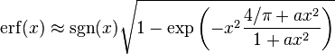
where
This is designed to be very accurate in a neighborhood of 0 and a neighborhood of infinity, and the error is less than 0.00035 for all x. Using the alternate value a ≈ 0.147 reduces the maximum error to about 0.00012.[11]
This approximation can also be inverted to calculate the inverse error function:
Exponential bounds and a pure exponential approximation for the complementary error function are given by [12]

A single-term lower bound is [13]
where the parameter β can be picked to minimize error on the desired interval of approximation.
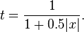
Numerical approximation
Over the complete range of values, there is an approximation with a maximal error of  , as follows:[14]
with
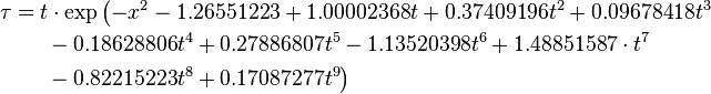
and
Applications
When the results of a series of measurements are described by a normal distribution with standard deviation  and expected value 0, then
  is the probability that the error of a single measurement lies between −a and +a, for positive a. This is useful, for example, in determining the bit error rate of a digital communication system.
The error and complementary error functions occur, for example, in solutions of the heat equation when boundary conditions are given by the Heaviside step function.
The error function and its approximations can be used to estimate results that hold with high probability. Given random variable ![X \sim Norm[\mu,\sigma]](../I/m/61aa404765b90f298a404db57647d45d.png) and constant
and constant  :
:
![Prob[X\leq L] = \frac{1}{2} + \frac{1}{2}\operatorname{erf}(\frac{L-\mu}{\sqrt{2}\sigma}) \approx A \exp (-B (\frac{L-\mu}{\sigma})^2)](../I/m/71eed1df1a9ef5e0bc41a62116fe5372.png)
Where A and B are certain numeric constants. If L is sufficiently far from the mean, i.e.  , then:
![Prob[X\leq L] \leq A \exp (-B \ln{k}) = \frac{A}{k^B}](../I/m/c3083d130dc0ccab2db2295362fed436.png)
so the probability goes to 0 as  .
.
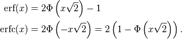
Related functions
The error function is essentially identical to the standard normal cumulative distribution function, denoted Φ, also named norm(x) by software languages, as they differ only by scaling and translation. Indeed,
![\Phi(x) =\frac{1}{\sqrt{2\pi}}\int_{-\infty}^x e^\tfrac{-t^2}{2}\,\mathrm dt = \frac{1}{2}\left[1+\operatorname{erf}\left(\frac{x}{\sqrt{2}}\right)\right]=\frac{1}{2}\,\operatorname{erfc}\left(-\frac{x}{\sqrt{2}}\right)](../I/m/84e78e72c2de2c238ff64c87396b135d.png)
or rearranged for erf and erfc:
Consequently, the error function is also closely related to the Q-function, which is the tail probability of the standard normal distribution. The Q-function can be expressed in terms of the error function as
The inverse of  is known as the normal quantile function, or probit function and may be expressed in terms of the inverse error function as

The standard normal cdf is used more often in probability and statistics, and the error function is used more often in other branches of mathematics.
The error function is a special case of the Mittag-Leffler function, and can also be expressed as a confluent hypergeometric function (Kummer's function):
It has a simple expression in terms of the Fresnel integral.
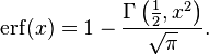
In terms of the regularized Gamma function P and the incomplete gamma function,
 is the sign function.
Generalized error functions

grey curve: E1(x) = (1 − e −x)/

red curve: E2(x) = erf(x)
green curve: E3(x)
blue curve: E4(x)
gold curve: E5(x).
Some authors discuss the more general functions:
Notable cases are:
- E0(x) is a straight line through the origin:

- E2(x) is the error function, erf(x).
After division by n!, all the En for odd n look similar (but not identical) to each other. Similarly, the En for even n look similar (but not identical) to each other after a simple division by n!. All generalised error functions for n > 0 look similar on the positive x side of the graph.
These generalised functions can equivalently be expressed for x > 0 using the Gamma function and incomplete Gamma function:
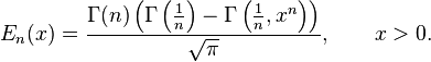
Therefore, we can define the error function in terms of the incomplete Gamma function:
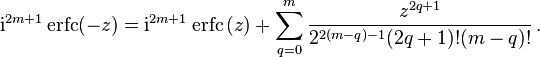
Iterated integrals of the complementary error function
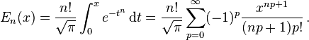
The iterated integrals of the complementary error function are defined by
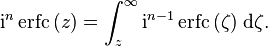
They have the power series
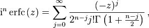
from which follow the symmetry properties
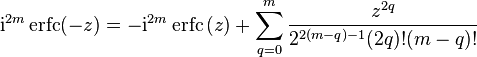
and
Implementations
- C: C99 provides the functions
double erf(double x)anddouble erfc(double x)in the header math.h. The pairs of functions {erff(),erfcf()} and {erfl(),erfcl()} take and return values of typefloatandlong doublerespectively. Forcomplex doublearguments, the function namescerfandcerfcare "reserved for future use"; the missing implementation is provided by the open-source project libcerf, which is based on the Faddeeva package.
- C++: C++11 provides
erf()anderfc()in the headercmath. Both functions are overloaded to accept arguments of typefloat,double, andlong double. Forcomplex<double>, the Faddeeva package provides a C++complex<double>implementation.
- Excel: Microsoft Excel provides the
erf, and theerfcfunctions, nonetheless both inverse functions are not in the current library.[15]
- Fortran: The Fortran 2008 standard provides the
ERF,ERFCandERFC_SCALEDfunctions to calculate the error function and its complement for real arguments. Fortran 77 implementations are available in SLATEC.
- Google search: Google's search also acts as a calculator and will evaluate "erf(...)" and "erfc(...)" for real arguments.
- Haskell: An erf package[16] exists that provides a typeclass for the error function and implementations for the native (real) floating point types.
- IDL: provides both erf and erfc for real and complex arguments.
- Julia: Includes
erfanderfcfor real and complex arguments. Also haserfifor calculating
- Maple: Maple implements both erf and erfc for real and complex arguments.
- MathCAD provides both erf(x) and erfc(x) for real arguments.
- Mathematica: erf is implemented as Erf and Erfc in Mathematica for real and complex arguments, which are also available in Wolfram Alpha.
- Matlab provides both erf and erfc for real arguments, also via W. J. Cody's algorithm.[18]
- Maxima provides both erf and erfc for real and complex arguments.
- PARI/GP: provides erfc for real and complex arguments, via tanh-sinh quadrature plus special cases.
- Perl: erf (for real arguments, using Cody's algorithm[18]) is implemented in the Perl module Math::SpecFun
- Python: Included since version 2.7 as
math.erf()for real arguments. For previous versions or for complex arguments, SciPy includes implementations of erf, erfc, erfi, and related functions for complex arguments inscipy.special.[19] A complex-argument erf is also in the arbitrary-precision arithmetic mpmath library asmpmath.erf()
- R: "The so-called 'error function'"[20] is not provided directly, but is detailed as an example of the normal cumulative distribution function (
?pnorm), which is based on W. J. Cody's rational Chebyshev approximation algorithm.[18]
- Ruby: Provides
Math.erf()andMath.erfc()for real arguments.
See also
Related functions
- Gaussian integral, over the whole real line
- Gaussian function, derivative
- Dawson function, renormalized imaginary error function
- Goodwin–Staton integral
In probability
- Normal distribution
- Normal cumulative distribution function, a scaled and shifted form of error function
- Probit, the inverse or quantile function of the normal CDF
- Q-function, the tail probability of the normal distribution
References
- ↑ Andrews, Larry C.; Special functions of mathematics for engineers
- ↑ 2.0 2.1 Greene, William H.; Econometric Analysis (fifth edition), Prentice-Hall, 1993, p. 926, fn. 11
- ↑ 3.0 3.1 3.2 Cody, W. J. (March 1993), "Algorithm 715: SPECFUN—A portable FORTRAN package of special function routines and test drivers" (PDF), ACM Trans. Math. Soft. 19 (1): 22–32, doi:10.1145/151271.151273
- ↑ Zaghloul, M. R. (March 1, 2007), "On the calculation of the Voigt line profile: a single proper integral with a damped sine integrand", Monthly Notices of the Royal Astronomical Society 375 (3): 1043–1048, doi:10.1111/j.1365-2966.2006.11377.x
- ↑ John W. Craig, A new, simple and exact result for calculating the probability of error for two-dimensional signal constellaions, Proc. 1991 IEEE Military Commun. Conf., vol. 2, pp. 571–575.
- ↑ Van Zeghbroeck, Bart; Principles of Semiconductor Devices, University of Colorado, 2011.
- ↑ Wolfram MathWorld
- ↑ H. M. Schöpf and P. H. Supancic, "On Bürmann's Theorem and Its Application to Problems of Linear and Nonlinear Heat Transfer and Diffusion," The Mathematica Journal, 2014. doi:10.3888/tmj.16–11.Schöpf, Supancic
- ↑ E. W. Weisstein. "Bürmann's Theorem" from Wolfram MathWorld—A Wolfram Web Resource./ E. W. Weisstein
- ↑ Cuyt, Annie A. M.; Petersen, Vigdis B.; Verdonk, Brigitte; Waadeland, Haakon; Jones, William B. (2008). Handbook of Continued Fractions for Special Functions. Springer-Verlag. ISBN 978-1-4020-6948-2.
- ↑ Winitzki, Sergei (6 February 2008). "A handy approximation for the error function and its inverse" (PDF). Retrieved 2011-10-03.
- ↑ Chiani, M., Dardari, D., Simon, M.K. (2003). New Exponential Bounds and Approximations for the Computation of Error Probability in Fading Channels. IEEE Transactions on Wireless Communications, 4(2), 840–845, doi=10.1109/TWC.2003.814350.
- ↑ Chang, Seok-Ho; Cosman, Pamela C.; Milstein, Laurence B. (November 2011). "Chernoff-Type Bounds for the Gaussian Error Function". IEEE Transactions on Communications 59 (11): 2939–2944. doi:10.1109/TCOMM.2011.072011.100049.
- ↑ Numerical Recipes in Fortran 77: The Art of Scientific Computing (ISBN 0-521-43064-X), 1992, page 214, Cambridge University Press.
- ↑ These results can however be obtained using the
NormSInvfunction as follows:erf_inverse(p) = -NormSInv((1 - p)/2)/SQRT(2);erfc_inverse(p) = -NormSInv(p/2)/SQRT(2). See . - ↑ http://hackage.haskell.org/package/erf
- ↑ Commons Math: The Apache Commons Mathematics Library
- ↑ 18.0 18.1 18.2 Cody, William J. (1969). "Rational Chebyshev Approximations for the Error Function" (PDF). Math. Comp. 23 (107): 631–637. doi:10.1090/S0025-5718-1969-0247736-4.
- ↑ Error Function and Fresnel Integrals, SciPy v0.13.0 Reference Guide.
- ↑ R Development Core Team (25 February 2011), R: The Normal Distribution
- Abramowitz, Milton; Stegun, Irene A., eds. (1965), "Chapter 7", Handbook of Mathematical Functions with Formulas, Graphs, and Mathematical Tables, New York: Dover, p. 297, ISBN 978-0486612720, MR 0167642.
- Press, William H.; Teukolsky, Saul A.; Vetterling, William T.; Flannery, Brian P. (2007), "Section 6.2. Incomplete Gamma Function and Error Function", Numerical Recipes: The Art of Scientific Computing (3rd ed.), New York: Cambridge University Press, ISBN 978-0-521-88068-8
- Temme, Nico M. (2010), "Error Functions, Dawson’s and Fresnel Integrals", in Olver, Frank W. J.; Lozier, Daniel M.; Boisvert, Ronald F.; Clark, Charles W., NIST Handbook of Mathematical Functions, Cambridge University Press, ISBN 978-0521192255, MR 2723248