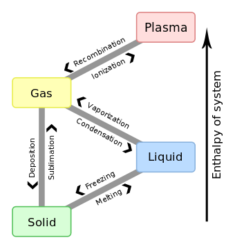
Enthalpy of fusion
The enthalpy of fusion also known as (latent) heat of fusion is the change in enthalpy resulting from heating a given quantity of a substance to change its state from a solid to a liquid. The temperature at which this occurs is the melting point.
The 'enthalpy' of fusion is a latent heat, because during melting the introduction of heat cannot be observed as a temperature change, as the temperature remains constant during the process. The latent heat of fusion is the enthalpy change of any amount of substance when it melts. When the heat of fusion is referenced to a unit of mass, it is usually called the specific heat of fusion, while the molar heat of fusion refers to the enthalpy change per amount of substance in moles.
The liquid phase has a higher internal energy than the solid phase. This means energy must be supplied to a solid in order to melt it and energy is released from a liquid when it freezes, because the molecules in the liquid experience weaker intermolecular forces and so have a higher potential energy (a kind of bond-dissociation energy for intermolecular forces).
When liquid water is cooled, its temperature falls steadily until it drops just below the line of freezing point at 0 °C. The temperature then remains constant at the freezing point while the water crystallizes. Once the water is completely frozen, its temperature continues to fall.
The enthalpy of fusion is almost always a positive quantity; helium is the only known exception.[1] Helium-3 has a negative enthalpy of fusion at temperatures below 0.3 K. Helium-4 also has a very slightly negative enthalpy of fusion below 0.8 K. This means that, at appropriate constant pressures, these substances freeze with the addition of heat.[2]
Reference values of common substances


| Substance | Heat of fusion (cal/g) |
Heat of fusion (J/g) |
|---|---|---|
| water | 79.97 | 334.774 |
| methane | 13.96 | 58.99 |
| propane | 19.11 | 79.96 |
| glycerol | 47.95 | 200.62 |
| formic acid | 66.05 | 276.35 |
| acetic acid | 45.90 | 192.09 |
| acetone | 23.42 | 97.99 |
| benzene | 30.45 | 127.40 |
| myristic acid | 47.49 | 198.70 |
| palmitic acid | 39.18 | 163.93 |
| stearic acid | 47.54 | 198.91 |
| Paraffin wax (C25H52) | 47.8-52.6 | 200–220 |
These values are from the CRC Handbook of Chemistry and Physics, 62nd edition. The conversion between cal/g and J/g in the above table uses the thermochemical calorie (calth) = 4.184 joules rather than the International Steam Table calorie (calINT) = 4.1868 joules.
Applications
1) To heat one kilogram (about 1 liter) of water from 283.15 K to 303.15 K (10 °C to 30 °C) requires 83.6 kJ.
However, to melt ice and raise the resulting water temperature by 20 K requires extra energy. To heat ice from 273.15 K to water at 293.15 K (0 °C to 20 °C) requires:
- (1) 333.55 J/g (heat of fusion of ice) = 333.55 kJ/kg = 333.55 kJ for 1 kg of ice to melt
- PLUS
- (2) 4.18 J/(g·K)· 20K = 4.18 kJ/(kg·K)· 20K = 83.6 kJ for 1kg of water to go up 20 K
- = 417.15 kJ
Or to restate it in everyday terms, one part ice at 0 °C will cool almost exactly 4 parts water at 20 °C to 0 °C.
2) Silicon has a heat of fusion of 50.21 kJ/mol. 50 kW of power can supply the energy required to melt about 100 kg of silicon in one hour, after it is brought to the melting point temperature:
50 kW = 50kJ/s = 180000kJ/h
180000kJ/h * (1 mol Si)/50.21kJ * 28gSi/(mol Si) * 1kgSi/1000gSi = 100.4kg/h
Solubility prediction
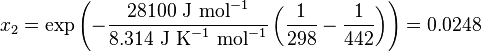
The heat of fusion can also be used to predict solubility for solids in liquids. Provided an ideal solution is obtained the mole fraction  of solute at saturation is a function of the heat of fusion, the melting point of the solid
  and the temperature (T) of the solution:

Here, R is the gas constant. For example the solubility of paracetamol in water at 298 K is predicted to be:
This equals to a solubility in grams per liter of:
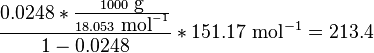
which is a deviation from the real solubility (240 g/L) of 11%. This error can be reduced when an additional heat capacity parameter is taken into account[3]
Proof
At equilibrium the chemical potentials for the pure solvent and pure solid are identical:

or

with  the gas constant and
  the temperature.
Rearranging gives:

and since

the heat of fusion being the difference in chemical potential between the pure liquid and the pure solid, it follows that

Application of the Gibbs–Helmholtz equation:
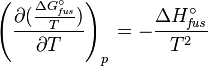
ultimately gives:
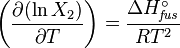
or:
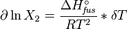
and with integration:
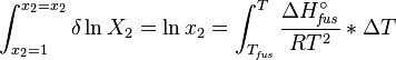
the end result is obtained:
See also
- Heat of vaporization
- Heat capacity
- Thermodynamic databases for pure substances
- Joback method (Estimation of the heat of fusion from molecular structure)
- Latent heat
Notes
- ↑ Atkins & Jones 2008, p. 236.
- ↑ Ott & Boerio-Goates 2000, pp. 92–93.
- ↑ Measurement and Prediction of Solubility of Paracetamol in Water-Isopropanol Solution. Part 2. Prediction H. Hojjati and S. Rohani Org. Process Res. Dev.; 2006; 10(6) pp 1110–1118; (Article) doi:10.1021/op060074g
References
- Atkins, Peter; Jones, Loretta (2008), Chemical Principles: The Quest for Insight (4th ed.), W. H. Freeman and Company, p. 236, ISBN 0-7167-7355-4
- Ott, J. Bevan; Boerio-Goates, Juliana (2000), Chemical Thermodynamics: Advanced Applications, Academic Press, ISBN 0-12-530985-6
| ||||||||||||||||||||||||||||||||||||