Elliptic cylindrical coordinates
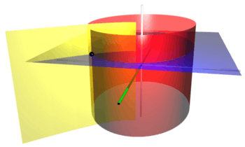
Elliptic cylindrical coordinates are a three-dimensional orthogonal coordinate system that results from projecting the two-dimensional elliptic coordinate system in the
perpendicular  -direction. Hence, the coordinate surfaces are prisms of confocal ellipses and hyperbolae. The two foci
 and
and  are generally taken to be fixed at
  and
and
 , respectively, on the
  -axis of the Cartesian coordinate system.
Basic definition
The most common definition of elliptic cylindrical coordinates  is
is


where  is a nonnegative real number and
  .
.
These definitions correspond to ellipses and hyperbolae. The trigonometric identity
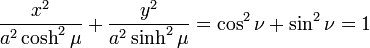
shows that curves of constant form ellipses, whereas the hyperbolic trigonometric identity
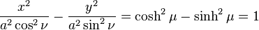
shows that curves of constant  form hyperbolae.
Scale factors
The scale factors for the elliptic cylindrical coordinates and are equal
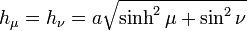
whereas the remaining scale factor  .
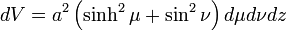
Consequently, an infinitesimal volume element equals
.
Consequently, an infinitesimal volume element equals
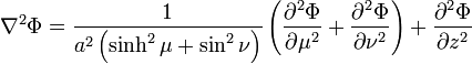
and the Laplacian equals
Other differential operators such as  and
and  can be expressed in the coordinates by substituting
the scale factors into the general formulae found in orthogonal coordinates.
can be expressed in the coordinates by substituting
the scale factors into the general formulae found in orthogonal coordinates.
Alternative definition
An alternative and geometrically intuitive set of elliptic coordinates  are sometimes used, where
  and
and  . Hence, the curves of constant
  are ellipses, whereas the curves of constant
  are hyperbolae. The coordinate must belong to the interval [-1, 1], whereas the
coordinate must be greater than or equal to one.
are hyperbolae. The coordinate must belong to the interval [-1, 1], whereas the
coordinate must be greater than or equal to one.
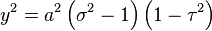
The coordinates have a simple relation to the distances to the foci and . For any point in the (x,y) plane, the sum  of its distances to the foci equals
  , whereas their difference
  equals
  .
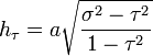
Thus, the distance to is
.
Thus, the distance to is  , whereas the distance to is
  . (Recall that and are located at
  and
and  , respectively.)
A drawback of these coordinates is that they do not have a 1-to-1 transformation to the Cartesian coordinates

Alternative scale factors
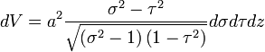
The scale factors for the alternative elliptic coordinates are
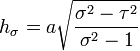
and, of course, . Hence, the infinitesimal volume element becomes
and the Laplacian equals
![\nabla^{2} \Phi =
\frac{1}{a^{2} \left( \sigma^{2} - \tau^{2} \right) }
\left[
\sqrt{\sigma^{2} - 1} \frac{\partial}{\partial \sigma}
\left( \sqrt{\sigma^{2} - 1} \frac{\partial \Phi}{\partial \sigma} \right) +
\sqrt{1 - \tau^{2}} \frac{\partial}{\partial \tau}
\left( \sqrt{1 - \tau^{2}} \frac{\partial \Phi}{\partial \tau} \right)
\right] +
\frac{\partial^{2} \Phi}{\partial z^{2}}](../I/m/efae343374068d4af8397e0c8ad55c03.png)
Other differential operators such as
and can be expressed in the coordinates  by substituting
the scale factors into the general formulae
found in orthogonal coordinates.
by substituting
the scale factors into the general formulae
found in orthogonal coordinates.
Applications
The classic applications of elliptic cylindrical coordinates are in solving partial differential equations,
e.g., Laplace's equation or the Helmholtz equation, for which elliptic cylindrical coordinates allow a
separation of variables. A typical example would be the electric field surrounding a
flat conducting plate of width  .
.
The three-dimensional wave equation, when expressed in elliptic cylindrical coordinates, may be solved by separation of variables, leading to the Mathieu differential equations.
The geometric properties of elliptic coordinates can also be useful. A typical example might involve
an integration over all pairs of vectors  and
and  that sum to a fixed vector
  , where the integrand
was a function of the vector lengths
, where the integrand
was a function of the vector lengths  and
and  . (In such a case, one would position
  between the two foci and aligned with the -axis, i.e.,
  .) For concreteness, , and could represent the momenta of a particle and its decomposition products, respectively, and the integrand might involve the kinetic energies of the products (which are proportional to the squared lengths of the momenta).
Bibliography
- Morse PM, Feshbach H (1953). Methods of Theoretical Physics, Part I. New York: McGraw-Hill. p. 657. ISBN 0-07-043316-X. LCCN 52011515.
- Margenau H, Murphy GM (1956). The Mathematics of Physics and Chemistry. New York: D. van Nostrand. pp. 182–183. LCCN 55010911.
- Korn GA, Korn TM (1961). Mathematical Handbook for Scientists and Engineers. New York: McGraw-Hill. p. 179. LCCN 59014456. ASIN B0000CKZX7.
- Sauer R, Szabó I (1967). Mathematische Hilfsmittel des Ingenieurs. New York: Springer Verlag. p. 97. LCCN 67025285.
- Zwillinger D (1992). Handbook of Integration. Boston, MA: Jones and Bartlett. p. 114. ISBN 0-86720-293-9. Same as Morse & Feshbach (1953), substituting uk for ξk.
- Moon P, Spencer DE (1988). "Elliptic-Cylinder Coordinates (η, ψ, z)". Field Theory Handbook, Including Coordinate Systems, Differential Equations, and Their Solutions (corrected 2nd ed., 3rd print ed.). New York: Springer-Verlag. pp. 17–20 (Table 1.03). ISBN 978-0-387-18430-2.
External links
| ||||||||||