Eigenvalues and eigenvectors of the second derivative
Explicit formulas for eigenvalues and eigenvectors of the second derivative with different boundary conditions are provided both for the continuous and discrete cases. In the discrete case, the standard central difference approximation of the second derivative is used on a uniform grid.
These formulas are used to derive the expressions for eigenfunctions of Laplacian in case of separation of variables, as well as to find eigenvalues and eigenvectors of multidimensional discrete Laplacian on a regular grid, which is presented as a Kronecker sum of discrete Laplacians in one-dimension.
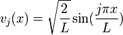
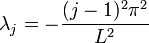
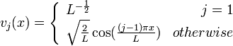
The continuous case
The index j represents the jth eigenvalue or eigenvector and runs from 1 to  . Assuming the equation is defined on the domain
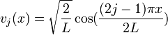
 ![x \in [0,L]](../I/m/624c78397df5054fd6a1e3b3c2bd2032.png) , the following are the eigenvalues and normalized eigenvectors. The eigenvalues are ordered in descending order.
, the following are the eigenvalues and normalized eigenvectors. The eigenvalues are ordered in descending order.
Pure Dirichlet boundary conditions

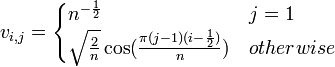
Pure Neumann boundary conditions
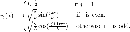
Periodic boundary conditions
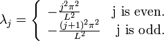
(That is:  is a simple eigenvalue and all further eigenvalues are given by
  ,
,  , each with multiplicity 2).
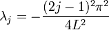
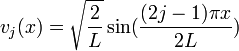
Mixed Dirichlet-Neumann boundary conditions
Mixed Neumann-Dirichlet boundary conditions
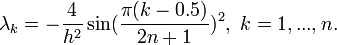
The discrete case
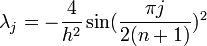
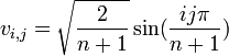
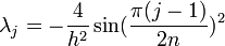
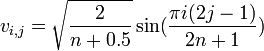
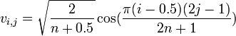
Notation: The index j represents the jth eigenvalue or eigenvector. The index i represents the ith component of an eigenvector. Both i and j go from 1 to n, where the matrix is size n x n. Eigenvectors are normalized. The eigenvalues are ordered in descending order.
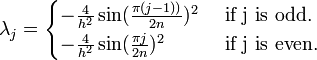
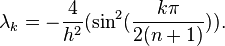
Pure Dirichlet boundary conditions
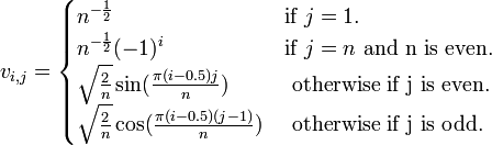
Pure Neumann boundary conditions
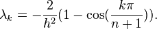
Periodic boundary conditions
(Note that eigenvalues are repeated except for 0 and the largest one if n is even.)
Mixed Dirichlet-Neumann boundary conditions
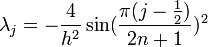
Mixed Neumann-Dirichlet boundary conditions
Derivation of Eigenvalues and Eigenvectors in the Discrete Case
Dirichlet case
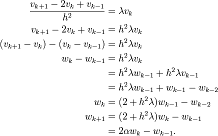
In the 1D discrete case with Dirichlet boundary conditions, we are solving

Rearranging terms, we get
Now let 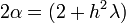 . Also, assuming
  , we can scale eigenvectors by any nonzero scalar, so scale
  so that
  .
.
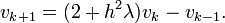
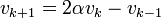
Then we find the recurrence


Considering  as an indeterminate,
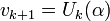
where  is the kth Chebyshev polynomial of the 2nd kind.
Since  , we get that
 .
.
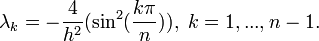
It is clear that the eigenvalues of our problem will be the zeros of the nth Chebyshev polynomial of the second kind, with the relation .
These zeros are well known and are:
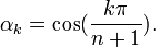
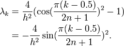
Plugging these into the formula for  ,
,
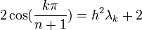
And using a trig formula to simplify, we find
Neumann case
In the Neumann case, we are solving

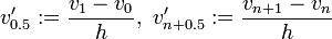
In the standard discretization, we introduce  and
and  and define
The boundary conditions are then equivalent to

If we make a change of variables,

we can derive the following:
with 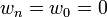 being the boundary conditions.
This is precisely the Dirichlet formula with  interior grid points and grid spacing
  . Similar to what we saw in the above, assuming
  , we get
This gives us eigenvalues and there are  . If we drop the assumption that , we find there is also a solution with
  and this corresponds to eigenvalue .
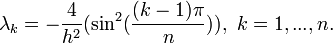
Relabeling the indices in the formula above and combining with the zero eigenvalue, we obtain,
Dirichlet-Neumann Case
For the Dirichlet-Neumann case, we are solving
 ,
,
where 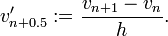
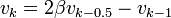
We need to introduce auxiliary variables 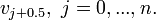
Consider the recurrence
 .
.
Also, we know  and assuming
  , we can scale
  so that
We can also write
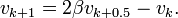
Taking the correct combination of these three equations, we can obtain
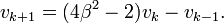
And thus our new recurrence will solve our eigenvalue problem when
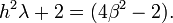
Solving for we get
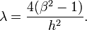
Our new recurrence gives

where  again is the kth Chebyshev polynomial of the 2nd kind.
And combining with our Neumann boundary condition, we have

A well-known formula relates the Chebyshev polynomials of the first kind,  , to those of the second kind by

Thus our eigenvalues solve
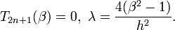
The zeros of this polynomial are also known to be
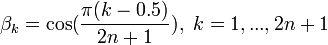
And thus
Note that there are 2n + 1 of these values, but only the first n + 1 are unique. The (n + 1)th value gives us the zero vector as an eigenvector with eigenvalue 0, which is trivial. This can be seen by returning to the original recurrence. So we consider only the first n of these values to be the n eigenvalues of the Dirichlet - Neumann problem.