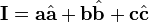
Dyadics

In multilinear algebra, a dyadic or dyadic tensor is a second order tensor written in a special notation, formed by juxtaposing pairs of vectors, along with a notation for manipulating such expressions analogous to the rules for matrix algebra. The notation and terminology are relatively obsolete today. Its uses in physics include continuum mechanics and electromagnetism.

Dyadic notation was first established by Josiah Willard Gibbs in 1884.

In this article, upper-case bold variables denote dyadics (including dyads) whereas lower-case bold variables denote vectors. An alternative notation uses respectively double and single over- or underbars.

Definitions and terminology

Dyadic, outer, and tensor products

A dyad is a tensor of order two and rank one, and is the result of the dyadic product of two vectors (complex vectors in general), whereas a dyadic is a general tensor of order two.

There are several equivalent terms and notations for this product:

the dyadic product of two vectors a and b is denoted by the juxtaposition ab,
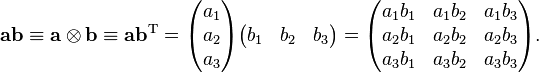
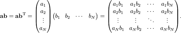
the outer product of two column vectors a and b is denoted and defined as a ⊗ b or ab^T, where T means transpose,
the tensor product of two vectors a and b is denoted a ⊗ b,

In the dyadic context they all have the same definition and meaning, and are used synonymously, although the tensor product is an instance of the more general and abstract use of the term.

Three-dimensional Euclidean space

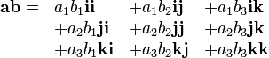
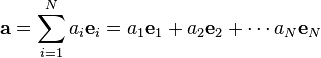
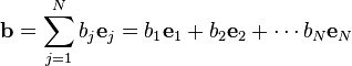
To illustrate the equivalent usage, consider three-dimensional Euclidean space, letting:

\mathbf{a} = a_1 \mathbf{i} + a_2 \mathbf{j} + a_3 \mathbf{k}

\mathbf{b} = b_1 \mathbf{i} + b_2 \mathbf{j} + b_3 \mathbf{k}

be two vectors where i, j, k (also denoted e₁, e₂, e₃) are the standard basis vectors in this vector space (see also Cartesian coordinates). Then the dyadic product of a and b can be represented as a sum:

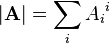
\begin{array}{llll} \mathbf{ab} = & a_1 b_1 \mathbf{i i} & + a_1 b_2 \mathbf{i j} & + a_1 b_3 \mathbf{i k} \\ &+ a_2 b_1 \mathbf{j i} & + a_2 b_2 \mathbf{j j} & + a_2 b_3 \mathbf{j k}\\ &+ a_3 b_1 \mathbf{k i} & + a_3 b_2 \mathbf{k j} & + a_3 b_3 \mathbf{k k} \end{array}

or by extension from row and column vectors, a 3×3 matrix (also the result of the outer product or tensor product of a and b):

\mathbf{a b} \equiv \mathbf{a}\otimes\mathbf{b} \equiv \mathbf{a b}^\mathrm{T} = \begin{pmatrix} a_1 \\ a_2 \\ a_3 \end{pmatrix}\begin{pmatrix} b_1 & b_2 & b_3 \end{pmatrix} = \begin{pmatrix} a_1b_1 & a_1b_2 & a_1b_3 \\ a_2b_1 & a_2b_2 & a_2b_3 \\ a_3b_1 & a_3b_2 & a_3b_3 \end{pmatrix}.

A dyad is a component of the dyadic (a monomial of the sum or equivalently entry of the matrix) - the juxtaposition of a pair of basis vectors scalar multiplied by a number.

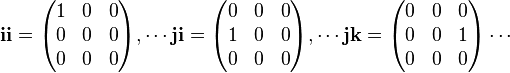
Just as the standard basis (and unit) vectors i, j, k, have the representations:

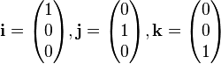
\mathbf{i} = \begin{pmatrix} 1 \\ 0 \\ 0 \end{pmatrix}, \mathbf{j} = \begin{pmatrix} 0 \\ 1 \\ 0 \end{pmatrix}, \mathbf{k} = \begin{pmatrix} 0 \\ 0 \\ 1 \end{pmatrix}

(which can be transposed), the standard basis (and unit) dyads have the representation:

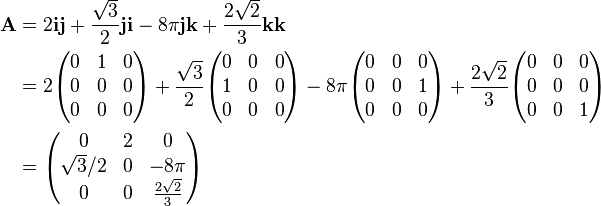
\mathbf{ii} = \begin{pmatrix} 1 & 0 & 0 \\ 0 & 0 & 0 \\ 0 & 0 & 0 \end{pmatrix}, \cdots \mathbf{ji} = \begin{pmatrix} 0 & 0 & 0 \\ 1 & 0 & 0 \\ 0 & 0 & 0 \end{pmatrix}, \cdots \mathbf{jk} = \begin{pmatrix} 0 & 0 & 0 \\ 0 & 0 & 1 \\ 0 & 0 & 0 \end{pmatrix} \cdots

For a simple numerical example in the standard basis:

\begin{align} \mathbf{A} & = 2\mathbf{ij} + \frac{\sqrt{3}}{2}\mathbf{ji} - 8\pi \mathbf{jk} + \frac{2\sqrt{2}}{3} \mathbf{kk} \\ & = 2 \begin{pmatrix} 0 & 1 & 0 \\ 0 & 0 & 0 \\ 0 & 0 & 0 \end{pmatrix} + \frac{\sqrt{3}}{2}\begin{pmatrix} 0 & 0 & 0 \\ 1 & 0 & 0 \\ 0 & 0 & 0 \end{pmatrix} - 8\pi \begin{pmatrix} 0 & 0 & 0 \\ 0 & 0 & 1 \\ 0 & 0 & 0 \end{pmatrix} + \frac{2\sqrt{2}}{3}\begin{pmatrix} 0 & 0 & 0 \\ 0 & 0 & 0 \\ 0 & 0 & 1 \end{pmatrix}\\ & = \begin{pmatrix} 0 & 2 & 0 \\ \sqrt{3}/2 & 0 & - 8\pi \\ 0 & 0 & \frac{2\sqrt{2}}{3} \end{pmatrix} \end{align}

N-dimensional Euclidean space

If the Euclidean space is N-dimensional, and

\mathbf{a} = \sum_{i=1}^N a_i\mathbf{e}_i = a_1 \mathbf{e}_1 + a_2 \mathbf{e}_2 + \cdots a_N \mathbf{e}_N

\mathbf{b} = \sum_{j=1}^N b_j\mathbf{e}_j = b_1 \mathbf{e}_1 + b_2 \mathbf{e}_2 + \cdots b_N \mathbf{e}_N

where e_i and e_j are the standard basis vectors in N-dimensions (the index i on e_i selects a specific vector, not a component of the vector as in a_i), then in algebraic form their dyadic product is:

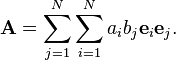
\mathbf{A} = \sum _{j=1}^N\sum_{i=1}^N a_ib_j{\mathbf{e}}_i\mathbf{e}_j.

This is known as the nonion form of the dyadic. Their outer/tensor product in matrix form is:

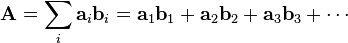
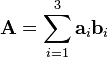
\mathbf{ab} = \mathbf{ab}^\mathrm{T} = \begin{pmatrix} a_1 \\ a_2 \\ \vdots \\ a_N \end{pmatrix}\begin{pmatrix} b_1 & b_2 & \cdots & b_N \end{pmatrix} = \begin{pmatrix} a_1b_1 & a_1b_2 & \cdots & a_1b_N \\ a_2b_1 & a_2b_2 & \cdots & a_2b_N \\ \vdots & \vdots & \ddots & \vdots \\ a_Nb_1 & a_Nb_2 & \cdots & a_Nb_N \end{pmatrix}.

A dyadic polynomial A, otherwise known as a dyadic, is formed from multiple vectors a_i and b_j:

\mathbf{A} = \sum_i\mathbf{a}_i\mathbf{b}_i = \mathbf{a}_1\mathbf{b}_1+\mathbf{a}_2\mathbf{b}_2+\mathbf{a}_3\mathbf{b}_3+\cdots

A dyadic which cannot be reduced to a sum of less than N dyads is said to be complete. In this case, the forming vectors are non-coplanar, see Chen (1983).

Classification

The following table classifies dyadics:

	Determinant	Adjugate	Matrix and its rank
Zero	= 0	= 0	= 0; rank 0: all zeroes
Linear	= 0	= 0	≠ 0; rank 1: at least one non-zero element and all 2 × 2 subdeterminants zero (single dyadic)
Planar	= 0	≠ 0 (single dyadic)	≠ 0; rank 2: at least one non-zero 2 × 2 subdeterminant
Complete	≠ 0	≠ 0	≠ 0; rank 3: non-zero determinant

Identities

The following identities are a direct consequence of the definition of the tensor product:^[1]

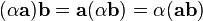
Compatible with scalar multiplication:
$(\alpha \mathbf{a}) \mathbf{b} =\mathbf{a} (\alpha \mathbf{b}) = \alpha (\mathbf{a} \mathbf{b})$
for any scalar $\alpha$ .
Distributive over vector addition:
$\mathbf{a} (\mathbf{b} + \mathbf{c}) =\mathbf{a} \mathbf{b} + \mathbf{a} \mathbf{c}$

$(\mathbf{a} + \mathbf{b}) \mathbf{c} =\mathbf{a} \mathbf{c} + \mathbf{b} \mathbf{c}$

Dyadic algebra

Product of dyadic and vector

There are four operations defined on a vector and dyadic, constructed from the products defined on vectors.

	Left	Right
Dot product	$\mathbf{c}\cdot \mathbf{a} \mathbf{b} = \left(\mathbf{c}\cdot\mathbf{a}\right)\mathbf{b}$	$\left(\mathbf{a}\mathbf{b}\right)\cdot \mathbf{c} = \mathbf{a}\left(\mathbf{b}\cdot\mathbf{c}\right)$
Cross product	$\mathbf{c} \times \left(\mathbf{ab}\right) = \left(\mathbf{c}\times\mathbf{a}\right)\mathbf{b}$	$\left(\mathbf{ab}\right)\times\mathbf{c} = \mathbf{a}\left(\mathbf{b}\times\mathbf{c}\right)$

Product of dyadic and dyadic

There are five operations for a dyadic to another dyadic. Let a, b, c, d be vectors. Then:

		Dot	Cross
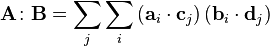
Dot	Dot product $\left(\mathbf{a}\mathbf{b}\right)\cdot\left(\mathbf{c}\mathbf{d}\right) = \mathbf{a}\left(\mathbf{b}\cdot\mathbf{c}\right)\mathbf{d}= \left(\mathbf{b}\cdot\mathbf{c}\right)\mathbf{a}\mathbf{d}$	Double dot product $\mathbf{ab}\colon\mathbf{cd}=\left(\mathbf{a}\cdot\mathbf{d}\right)\left(\mathbf{b}\cdot\mathbf{c}\right)$ or $\left(\mathbf{ab}\right):\left(\mathbf{cd}\right) = \mathbf{c}\cdot\left(\mathbf{ab}\right)\cdot\mathbf{d} = \left(\mathbf{a}\cdot\mathbf{c}\right)\left(\mathbf{b}\cdot\mathbf{d}\right)$	Dot–cross product $\left(\mathbf{ab}\right) \!\!\!\begin{array}{c} _\cdot \\ ^\times \end{array}\!\!\! \left(\mathbf{c}\mathbf{d}\right)=\left(\mathbf{a}\cdot\mathbf{c}\right)\left(\mathbf{b}\times\mathbf{d}\right)$
Cross		Cross–dot product $\left(\mathbf{ab}\right) \!\!\!\begin{array}{c} _\times \\ ^\cdot \end{array}\!\!\! \left(\mathbf{cd}\right)=\left(\mathbf{a}\times\mathbf{c}\right)\left(\mathbf{b}\cdot\mathbf{d}\right)$	Double cross product $\left(\mathbf{ab}\right) \!\!\!\begin{array}{c} _\times \\ ^\times \end{array}\!\!\! \left(\mathbf{cd}\right)=\left(\mathbf{a}\times\mathbf{c}\right)\left(\mathbf{b}\times \mathbf{d}\right)$

Letting

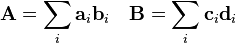
\mathbf{A}=\sum _i \mathbf{a}_i\mathbf{b}_i \quad \mathbf{B}=\sum _i \mathbf{c}_i\mathbf{d}_i

be two general dyadics, we have:

		Dot	Cross
Dot	Dot product 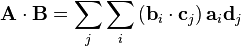$\mathbf{A}\cdot\mathbf{B} = \sum_j\sum _i\left(\mathbf{b}_i\cdot\mathbf{c}_j\right)\mathbf{a}_i\mathbf{d}_j$	Double dot product 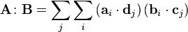$\mathbf{A}\colon\mathbf{B}=\sum_j\sum_i\left(\mathbf{a}_i\cdot\mathbf{d}_j\right)\left(\mathbf{b}_i\cdot\mathbf{c}_j\right)$ or $\mathbf{A}\colon\mathbf{B}=\sum_j\sum_i\left(\mathbf{a}_i\cdot\mathbf{c}_j\right)\left(\mathbf{b}_i\cdot\mathbf{d}_j\right)$	Dot–cross product 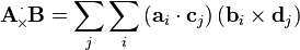$\mathbf{A}\!\!\!\begin{array}{c} _\cdot \\ ^\times \end{array}\!\!\! \mathbf{B} = \sum_j\sum _i \left(\mathbf{a}_i\cdot\mathbf{c}_j\right)\left(\mathbf{b}_i\times\mathbf{d}_j\right)$
Cross		Cross–dot product 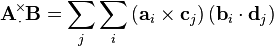$\mathbf{A}\!\!\!\begin{array}{c} _\times \\ ^\cdot \end{array}\!\!\! \mathbf{B} = \sum_j\sum _i \left(\mathbf{a}_i\times\mathbf{c}_j\right)\left(\mathbf{b}_i\cdot\mathbf{d}_j\right)$	Double cross product 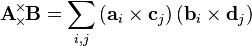$\mathbf{A} \!\!\!\begin{array}{c} _\times \\ ^\times \end{array}\!\!\! \mathbf{B}=\sum _{i,j} \left(\mathbf{a}_i\times \mathbf{c}_j\right)\left(\mathbf{b}_i\times \mathbf{d}_j\right)$

Double-dot product

There are two ways to define the double dot product, one must be careful when deciding which convention to use. As there are no analogous matrix operations for the remaining dyadic products, no ambiguities in their definitions appear.

The double-dot product is commutative due to commutativity of the normal dot-product:

\mathbf{A} \colon \! \mathbf{B} = \mathbf{B} \colon \! \mathbf{A}

There is a special double dot product with a transpose

\mathbf{A} \colon \! \mathbf{B}^\mathrm{T} = \mathbf{A}^\mathrm{T} \colon \! \mathbf{B}

Another identity is:

\mathbf{A}\colon\mathbf{B}=\left(\mathbf{A}\cdot\mathbf{B}^\mathrm{T}\right)\colon \mathbf{I} =\left(\mathbf{B}\cdot\mathbf{A}^\mathrm{T}\right)\colon \mathbf{I}

Double-cross product

We can see that, for any dyad formed from two vectors a and b, its double cross product is zero.

\left(\mathbf{ab}\right) \!\!\!\begin{array}{c} _\times \\ ^\times \end{array}\!\!\! \left(\mathbf{ab}\right)=\left(\mathbf{a}\times\mathbf{a}\right)\left(\mathbf{b}\times\mathbf{b}\right)= 0

However, by definition, a dyadic double-cross product on itself will generally be non-zero. For example, a dyadic A composed of six different vectors

\mathbf{A}=\sum _{i=1}^3 \mathbf{a}_i\mathbf{b}_i

has a non-zero self-double-cross product of

\mathbf{A} \!\!\!\begin{array}{c} _\times \\ ^\times \end{array}\!\!\! \mathbf{A} = 2 \left[\left(\mathbf{a}_1\times \mathbf{a}_2\right)\left(\mathbf{b}_1\times \mathbf{b}_2\right)+\left(\mathbf{a}_2\times \mathbf{a}_3\right)\left(\mathbf{b}_2\times \mathbf{b}_3\right)+\left(\mathbf{a}_3\times \mathbf{a}_1\right)\left(\mathbf{b}_3\times \mathbf{b}_1\right)\right]

Tensor contraction

Main article: Tensor contraction

The spur or expansion factor arises from the formal expansion of the dyadic in a coordinate basis by replacing each juxtaposition by a dot product of vectors:

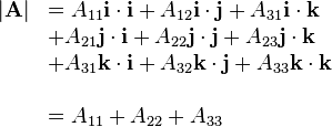
\begin{array}{llll} |\mathbf{A}| & = A_{11} \mathbf{i}\cdot\mathbf{i} + A_{12} \mathbf{i}\cdot\mathbf{j} + A_{31} \mathbf{i}\cdot\mathbf{k} \\ & + A_{21} \mathbf{j}\cdot\mathbf{i} + A_{22} \mathbf{j}\cdot\mathbf{j} + A_{23} \mathbf{j}\cdot\mathbf{k}\\ & + A_{31} \mathbf{k}\cdot\mathbf{i} + A_{32} \mathbf{k}\cdot\mathbf{j} + A_{33} \mathbf{k}\cdot\mathbf{k} \\ \\ & = A_{11} + A_{22} + A_{33} \\ \end{array}

in index notation this is the contraction of indices on the dyadic:

|\mathbf{A}| = \sum_i A_i{}^i

In three dimensions only, the rotation factor arises by replacing every juxtaposition by a cross product

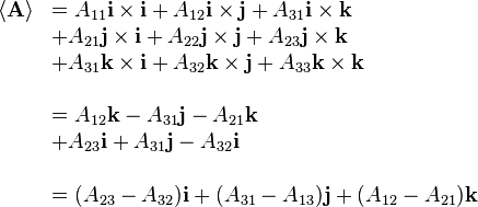
\begin{array}{llll} \langle\mathbf{A}\rangle & = A_{11} \mathbf{i}\times\mathbf{i} + A_{12} \mathbf{i}\times\mathbf{j} + A_{31} \mathbf{i}\times\mathbf{k} \\ & + A_{21} \mathbf{j}\times\mathbf{i} + A_{22} \mathbf{j}\times\mathbf{j} + A_{23} \mathbf{j}\times\mathbf{k}\\ & + A_{31} \mathbf{k}\times\mathbf{i} + A_{32} \mathbf{k}\times\mathbf{j} + A_{33} \mathbf{k}\times\mathbf{k} \\ \\ & = A_{12} \mathbf{k} - A_{31} \mathbf{j} - A_{21} \mathbf{k} \\ & + A_{23} \mathbf{i} + A_{31} \mathbf{j} - A_{32} \mathbf{i} \\ \\ & = (A_{23}-A_{32})\mathbf{i} + (A_{31}-A_{13})\mathbf{j} + (A_{12}-A_{21})\mathbf{k}\\ \end{array}

In index notation this is the contraction of A with the Levi-Civita tensor

\langle\mathbf{A}\rangle=\sum_{jk}{\epsilon_i}^{jk}A_{jk}.

Special dyadics

Unit dyadic

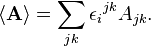
There exists a unit dyadic, denoted by I, such that, for any vector a,

\mathbf{I}\cdot\mathbf{a}=\mathbf{a}\cdot\mathbf{I}= \mathbf{a}

Given a basis of 3 vectors a, b and c, with reciprocal basis $\hat{{\mathbf{a}}}, \hat{\mathbf{b}}, \hat{\mathbf{c}}$ , the unit dyadic is expressed by

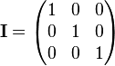
\mathbf{I} = \mathbf{a}\hat{\mathbf{a}} + \mathbf{b}\hat{\mathbf{b}} + \mathbf{c}\hat{\mathbf{c}}

In the standard basis,

\mathbf{I} = \mathbf{ii} + \mathbf{jj} + \mathbf{kk}

The corresponding matrix is

\mathbf{I}=\begin{pmatrix} 1 & 0 & 0\\ 0 & 1 & 0\\ 0 & 0 & 1\\ \end{pmatrix}

This can be put on more careful foundations (explaining what the logical content of "juxtaposing notation" could possibly mean) using the language of tensor products. If V is a finite-dimensional vector space, a dyadic tensor on V is an elementary tensor in the tensor product of V with its dual space.

The tensor product of V and its dual space is isomorphic to the space of linear maps from V to V: a dyadic tensor vf is simply the linear map sending any w in V to f(w)v. When V is Euclidean n-space, we can use the inner product to identify the dual space with V itself, making a dyadic tensor an elementary tensor product of two vectors in Euclidean space.

In this sense, the unit dyadic ij is the function from 3-space to itself sending a₁i + a₂j + a₃k to a₂i, and jj sends this sum to a‍₂j. Now it is revealed in what (precise) sense ii + jj + kk is the identity: it sends a₁i + a₂j + a₃k to itself because its effect is to sum each unit vector in the standard basis scaled by the coefficient of the vector in that basis.

Properties of unit dyadics

\left(\mathbf{a}\times\mathbf{I}\right)\cdot\left(\mathbf{b}\times\mathbf{I}\right)= \mathbf{ab}-\left(\mathbf{a}\cdot\mathbf{b}\right)\mathbf{I}

\mathbf{I} \!\!\begin{array}{c} _\times \\ ^\cdot \end{array}\!\!\! \left(\mathbf{ab}\right)=\mathbf{b}\times\mathbf{a}

\mathbf{I} \!\!\begin{array}{c} _\times \\ ^\times \end{array}\!\! \mathbf{A}=(\mathbf{A} \!\!\begin{array}{c} _\times \\ ^\times \end{array}\!\! \mathbf{I})\mathbf{I}-\mathbf{A}^\mathrm{T}

\mathbf{I}\;\colon\left(\mathbf{ab}\right) = \left(\mathbf{I}\cdot\mathbf{a}\right)\cdot\mathbf{b} = \mathbf{a}\cdot\mathbf{b} = \mathrm{tr}\left(\mathbf{ab}\right)

where "tr" denotes the trace.

Rotation dyadic

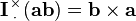
For any vector a in two dimensions, the left-cross product with the identity dyad I:

\mathbf{a}\times \mathbf{I}

is a 90 degree anticlockwise rotation dyadic around a. Alternatively the dyadic tensor

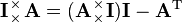
J = ji − ij =

\begin{pmatrix} 0 & -1 \\ 1 & 0 \end{pmatrix}

is a 90° anticlockwise rotation operator in 2d. It can be left-dotted with a vector to produce the rotation:

(\mathbf{j i} - \mathbf{i j}) \cdot (x \mathbf{i} + y \mathbf{j}) = x \mathbf{j i} \cdot \mathbf{i} - x \mathbf{i j} \cdot \mathbf{i} + y \mathbf{j i} \cdot \mathbf{j} - y \mathbf{i j} \cdot \mathbf{j} = -y \mathbf{i} + x \mathbf{j},

or in matrix notation

\begin{pmatrix} 0 & -1 \\ 1 & 0 \end{pmatrix} \begin{pmatrix} x \\ y \end{pmatrix}= \begin{pmatrix} -y \\ x \end{pmatrix}.

A general 2d rotation dyadic for θ angle anti-clockwise is

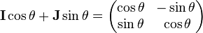
\mathbf{I}\cos\theta + \mathbf{J}\sin\theta = \begin{pmatrix} \cos\theta &-\sin\theta \\ \sin\theta &\;\cos\theta \end{pmatrix}

where I and J are as above.

Related terms

Some authors generalize from the term dyadic to related terms triadic, tetradic and polyadic.^[2]

References

↑ Spencer (1992), page 19.
↑ For example, I. V. Lindell and A. P. Kiselev (2001). "POLYADIC METHODS IN ELASTODYNAMICS". Progress In Electromagnetics Research, PIER 31: 113–154.

P. Mitiguy (2009). "Vectors and dyadics". Stanford, USA. Chapter 2
Spiegel, M.R.; Lipschutz, S.; Spellman, D. (2009). Vector analysis, Schaum's outlines. McGraw Hill. ISBN 978-0-07-161545-7.
A.J.M. Spencer (1992). Continuum Mechanics. Dover Publications. ISBN 0-486-43594-6. .
Morse, Philip M.; Feshbach, Herman (1953), "§1.6: Dyadics and other vector operators", Methods of theoretical physics, Volume 1, New York: McGraw-Hill, pp. 54–92, ISBN 978-0-07-043316-8, MR 0059774 .
Ismo V. Lindell (1996). Methods for Electromagnetic Field Analysis. Wiley-Blackwell. ISBN 978-0-7803-6039-6. .
Hollis C. Chen (1983). Theory of Electromagnetic Wave - A Coordinate-free approach. McGraw Hill. ISBN 978-0-07-010688-8. .

External links

Tensors

Glossary of tensor theory

Scope

Mathematics	coordinate system multilinear algebra Euclidean geometry tensor algebra differential geometry exterior calculus tensor calculus

Physics Engineering	continuum mechanics electromagnetism transport phenomena general relativity computer vision

Notation

Tensor definitions

Operations

Related abstractions

dimension
basis
vector, vector space
multivector
covariance and contravariance of vectors
linear transformation
matrix
spinor
Cartan formalism (physics)
differential form
exterior form
connection form
geodesic
manifold
fiber bundle

Notable tensors

Mathematics	Kronecker delta Levi-Civita symbol metric tensor nonmetricity tensor Christoffel symbols Ricci curvature Riemann curvature tensor Weyl tensor torsion tensor

Physics	moment of inertia angular momentum tensor spin tensor Cauchy stress tensor stress–energy tensor EM tensor gluon field strength tensor Einstein tensor metric tensor (GR)

Mathematicians