Design matrix

In statistics, a design matrix is a matrix of values of explanatory variables, often denoted by X, that is used in certain statistical models, e.g., the general linear model.^[1]^[2] It can contain indicator variables (ones and zeros) that indicate group membership in an ANOVA, or it can contain values of continuous variables.

The design matrix contains data on the independent variables (also called explanatory variables) in statistical models which attempt to explain observed data on a response variable (often called a dependent variable) in terms of the explanatory variables. The theory relating to such models makes substantial use of matrix manipulations involving the design matrix: see for example linear regression. A notable feature of the concept of a design matrix is that it is able to represent a number of different experimental designs and statistical models, e.g., ANOVA, ANCOVA, and linear regression.

Definition

In a regression model, written in matrix-vector form as

y=X\beta+ \epsilon,

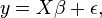
the matrix X is the design matrix, while y is the vector of observations on the dependent variable, $\beta$ is a vector of response coefficients (one for each explanatory variable) and $\epsilon$ is a vector containing the values of the model's error term for the various observations. In the design matrix, each column is a vector of observations on one of the explanatory variables.

Examples

Simple Regression

This section gives an example of simple linear regression—that is, regression with only a single explanatory variable—with seven observations. The seven data points are {y_i, x_i}, for i = 1, 2, …, 7. The simple linear regression model is

y_i = \beta_0 + \beta_1 x_i +\epsilon_i, \,

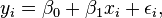
where $\beta_0$ is the y-intercept and $\beta_1$ is the slope of the regression line. This model can be represented in matrix form as

\begin{bmatrix}y_1 \\ y_2 \\ y_3 \\ y_4 \\ y_5 \\ y_6 \\ y_7 \end{bmatrix} = \begin{bmatrix}1 & x_1 \\1 & x_2 \\1 & x_3 \\1 & x_4 \\1 & x_5 \\1 & x_6 \\ 1 & x_7 \end{bmatrix} \begin{bmatrix} \beta_0 \\ \beta_1 \end{bmatrix} + \begin{bmatrix} \epsilon_1 \\ \epsilon_2 \\ \epsilon_3 \\ \epsilon_4 \\ \epsilon_5 \\ \epsilon_6 \\ \epsilon_7 \end{bmatrix}

where the first column of ones in the design matrix allows estimation of the y-intercept while the second column contains the x-values associated with the corresponding y-values.

Multiple Regression

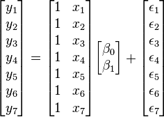
This section contains an example of multiple regression with two covariates (explanatory variables): w and x. Again suppose that the data consist of seven observations, and that for each observed value to be predicted ( $y_i$ ), values w_i and x_i of the two covariates are also observed. The model to be considered is

y_i = \beta_0 + \beta_1 w_i + \beta_2 x_i + \epsilon_i

This model can be written in matrix terms as

\begin{bmatrix}y_1 \\ y_2 \\ y_3 \\ y_4 \\ y_5 \\ y_6 \\ y_7 \end{bmatrix} = \begin{bmatrix} 1 & w_1 & x_1 \\1 & w_2 & x_2 \\1 & w_3 & x_3 \\1 & w_4 & x_4 \\1 & w_5 & x_5 \\1 & w_6 & x_6 \\ 1& w_7 & x_7 \end{bmatrix} \begin{bmatrix} \beta_0 \\ \beta_1 \\ \beta_2 \end{bmatrix} + \begin{bmatrix} \epsilon_1 \\ \epsilon_2 \\ \epsilon_3 \\ \epsilon_4 \\ \epsilon_5 \\ \epsilon_6 \\ \epsilon_7 \end{bmatrix}

Here the 7×3 matrix on the right side is the design matrix.

One-way ANOVA (Cell Means Model)

This section contains an example with a one-way analysis of variance (ANOVA) with three groups and seven observations. The given data set has the first three observations belonging to the first group, the following two observations belonging to the second group and the final two observations belonging to the third group. If the model to be fit is just the mean of each group, then the model is

y_{ij} = \mu_i + \epsilon_{ij}

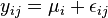
which can be written

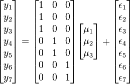
\begin{bmatrix}y_1 \\ y_2 \\ y_3 \\ y_4 \\ y_5 \\ y_6 \\ y_7 \end{bmatrix} = \begin{bmatrix}1 & 0 & 0 \\1 &0 &0 \\ 1 & 0 & 0 \\ 0 & 1 & 0 \\ 0 & 1 & 0 \\ 0 & 0 & 1 \\ 0 & 0 & 1\end{bmatrix} \begin{bmatrix}\mu_1 \\ \mu_2 \\ \mu_3 \end{bmatrix} + \begin{bmatrix} \epsilon_1 \\ \epsilon_2 \\ \epsilon_3 \\ \epsilon_4 \\ \epsilon_5 \\ \epsilon_6 \\ \epsilon_7 \end{bmatrix}

It should be emphasized that in this model $\mu_i$ represents the mean of the $i$ th group.

One-way ANOVA (offset from reference group)

The ANOVA model could be equivalently written as each group parameter $\tau_i$ being an offset from some overall reference. Typically this reference point is taken to be one of the groups under consideration. This makes sense in the context of comparing multiple treatment groups to a control group and the control group is considered the "reference". In this example, group 1 was chosen to be the reference group. As such the model to be fit is

y_{ij} = \mu + \tau_i + \epsilon_{ij}

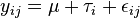
with the constraint that $\tau_1$ is zero.

\begin{bmatrix}y_1 \\ y_2 \\ y_3 \\ y_4 \\ y_5 \\ y_6 \\ y_7 \end{bmatrix} = \begin{bmatrix}1 &0 &0 \\1 &0 &0 \\ 1 & 0 & 0 \\ 1 & 1 & 0 \\ 1 & 1 & 0 \\ 1 & 0 & 1 \\ 1 & 0 & 1\end{bmatrix} \begin{bmatrix}\mu \\ \tau_2 \\ \tau_3 \end{bmatrix} + \begin{bmatrix} \epsilon_1 \\ \epsilon_2 \\ \epsilon_3 \\ \epsilon_4 \\ \epsilon_5 \\ \epsilon_6 \\ \epsilon_7 \end{bmatrix}

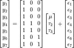
In this model $\mu$ is the mean of the reference group and $\tau_i$ is the difference from group $i$ to the reference group. $\tau_1$ is not included in the matrix because its difference from the reference group (itself) is necessarily zero.

References

↑ Everitt, B. S. (2002). Cambridge Dictionary of Statistics (2nd edition). Cambridge, UK: Cambridge University Press. ISBN 0-521-81099-X
↑ Box, G. E. P.; Tiao, G. C. (1992) [1973]. Bayesian Inference in Statistical Analysis. New York: John Wiley and Sons. ISBN 0-471-57428-7. (Section 8.1.1)