Degree of coherence
In quantum optics, correlation functions are used to characterize the statistical and coherence properties of an electromagnetic field. The degree of coherence is the normalized correlation of electric fields. In its simplest form, termed  , it is useful for quantifying the coherence between two electric fields, as measured in a Michelson or other linear optical interferometer. The correlation between pairs of fields,
  , typically is used to find the statistical character of intensity fluctuations. First order correlation is actually the amplitude-amplitude correlation and the second order correlation is the intensity-intensity correlation. It is also used to differentiate between states of light that require a quantum mechanical description and those for which classical fields are sufficient. Analogous considerations apply to any Bose field in subatomic physics, in particular to mesons (cf. Bose–Einstein correlations)
Degree of first-order coherence
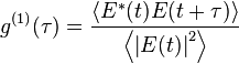
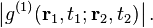
The normalized first order correlation function is written as:

![g^{(1)}( \mathbf{r}_1,t_1;\mathbf{r}_2,t_2)= \frac{\left \langle E^*(\mathbf{r}_1,t_1)E(\mathbf{r}_2,t_2) \right \rangle}{\left [ \left \langle\left | E(\mathbf{r}_1,t_1)\right |^2 \right \rangle \left \langle \left |E(\mathbf{r}_2,t_2)\right |^2 \right \rangle \right ]^{1/2}}](../I/m/83dbfb09bc53bec38213f50b35a96afb.png)
Where <> denotes an ensemble (statistical) average. For non-stationary states, such as pulses, the ensemble is made up of many pulses. When one deals with stationary states, where the statistical properties do not change with time, one can replace the ensemble average with a time average. If we restrict ourselves to plane parallel waves then  .
In this case, the result for stationary states will not depend on
.
In this case, the result for stationary states will not depend on  , but on the time delay
  (or
(or 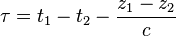 if
if  ).
).
This allows us to write a simplified form
 where we now average over t.
In optical interferometers such as the Michelson interferometer, Mach-Zehnder interferometer, or Sagnac interferometer, one splits an electric field into two components, introduces a time delay to one of the components, and then recombines them. The intensity of resulting field is measured as a function of the time delay. The visibility of the resulting interference pattern is given by  . More generally, when combining two space-time points from a field
- visibility=
The visibility ranges from zero, for incoherent electric fields, to one, for coherent electric fields. Anything in between is described as partially coherent.
Generally,  and
and 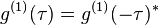 .
.
Examples of g(1)
For light of a single frequency (e.g. laser light): 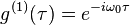
For Lorentzian chaotic light (e.g. collision broadened): 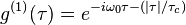
For Gaussian chaotic light (e.g. Doppler broadened): 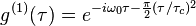
Here,  is the central frequency of the light and
  is the coherence time of the light.
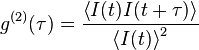
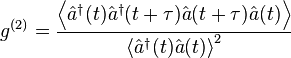
Degree of second-order coherence
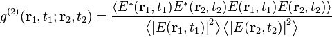
The normalised second order correlation function is written as:

Note that this is not a generalization of the first-order coherence
If the electric fields are considered classical, we can reorder them to express in terms of intensities. A plane parallel wave in a stationary state will have
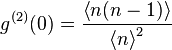
The above expression is even, 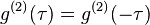 For classical fields, one can apply Cauchy-Schwarz inequality to the intensities in the above expression (since they are real numbers) to show that
 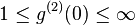 and that
 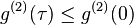 . Nevertheless the second-order coherence for an average over fringe of complementary interferometer outputs of a coherent state is only 0.5 (even though
  for each phase). And (calculated from averages) can be reduced down to zero with a proper discriminating trigger level applied to the signal (within the range of coherence).
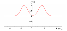
Examples of g(2)
Chaotic light of all kinds: 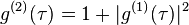 .
Note the Hanbury-Brown and Twiss effect uses this fact to find from a measurement of
.
Note the Hanbury-Brown and Twiss effect uses this fact to find from a measurement of  .
.
Light of a single frequency: 
Also, please see photon antibunching for another use of where  for a single photon source because
where  is the photon number observable.[1]
Degree of nth-order coherence
A generalization of the first-order coherence
![g^{(n)}( \mathbf{r}_1,t_1;\mathbf{r}_2,t_2;\dots;\mathbf{r}_{2n},t_{2n})= \frac{\left \langle E^*(\mathbf{r}_1,t_1)E^*(\mathbf{r}_2,t_2)\cdots E^*(\mathbf{r}_n,t_n)E(\mathbf{r}_{n+1},t_{n+1})E(\mathbf{r}_{n+2},t_{n+2}) \dots E(\mathbf{r}_{2n},t_{2n}) \right \rangle}{\left [ \left \langle\left | E(\mathbf{r}_1,t_1)\right |^2 \right \rangle \left \langle \left |E(\mathbf{r}_2,t_2)\right |^2 \right \rangle\cdots\left \langle \left |E(\mathbf{r}_{2n},t_{2n})\right |^2 \right \rangle \right ]^{1/2}}](../I/m/b18bd49c63a9faaeeb597ae3e59e2488.png)
A generalization of the second-order coherence

or in intensities

Examples of g(n)
Light of a single frequency:

Using the first definition:
Chaotic light of all kinds: 
Using the second definition:
Chaotic light of all kinds:  Chaotic light of all kinds:
Generalization to quantum fields

The predictions of  for n > 1 change when the classical fields (complex numbers or c-numbers) are replaced with quantum fields (operators or q-numbers). In general, quantum fields do not necessarily commute, with the consequence that their order in the above expressions can not be simply interchanged.


With
we get in the case of stationary light:
Photon bunching

Light is said to be bunched if 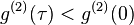 and antibunched if
  .
.
See also
- Bose–Einstein correlations
- Coherence theory
- Correlation and dependence
- Correlation does not imply causation
- Fourier transform spectroscopy
- Normally distributed and uncorrelated does not imply independent
- Optical autocorrelation
References
- ↑ SINGLE PHOTONS FOR QUANTUM INFORMATION PROCESSING - http://www.stanford.edu/group/yamamotogroup/Thesis/DFthesis.pdf
Suggested reading
- Loudon, Rodney, The Quantum Theory of Light (Oxford University Press, 2000), [ISBN 0-19-850177-3]