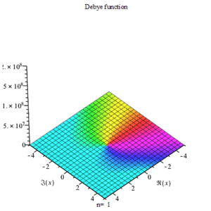
Debye function
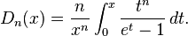
In mathematics, the family of Debye functions is defined by
The functions are named in honor of Peter Debye, who came across this function (with n = 3) in 1912 when he analytically computed the heat capacity of what is now called the Debye model.
Mathematical properties
Relation to other functions
The Debye functions are closely related to the Riemann zeta function and Polylogarithm
 :
:

Series Expansion
According to,[2]

Limiting values
For  :
:

For  :
:  is given by the Gamma function and the Riemann zeta function:
![D_n(x)\propto\int_0^\infty{\rm d}t\frac{t^{n}}{\exp(t)-1} = \Gamma(n + 1) \zeta(n + 1). \quad [\Re \, n > 0]](../I/m/e7a6f676add26b484d800fe976529979.png)
Applications in solid-state physics
The Debye model
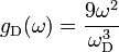
The Debye model has a density of vibrational states
 for
for 
with the Debye frequency ωD.
Internal energy and heat capacity
Inserting g into the internal energy
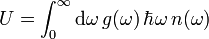
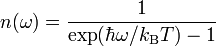
with the Bose–Einstein distribution
 .
.
one obtains
 .
.
The heat capacity is the derivative thereof.
Mean squared displacement
The intensity of X-ray diffraction or neutron diffraction at wavenumber q is given by the Debye-Waller factor or the Lamb-Mössbauer factor. For isotropic systems it takes the form
 ).
).
In this expression, the mean squared displacement refers to just once Cartesian component ux of the vector u that describes the displacement of atoms from their equilibrium positions. Assuming harmonicity and developing into normal modes,[4] one obtains
![2W(q)=\frac{\hbar^2 q^2}{6M k_{\rm B}T}\int_0^\infty{\rm d}\omega\frac{k_{\rm B}T}{\hbar\omega}g(\omega)\coth\frac{\hbar\omega}{2k_{\rm B}T}=\frac{\hbar^2 q^2}{6M k_{\rm B}T}\int_0^\infty{\rm d}\omega\frac{k_{\rm B}T}{\hbar\omega}g(\omega)\left[\frac{2}{\exp(\hbar\omega/k_{\rm B}T)-1}+1\right].](../I/m/0abccef6bf95ebcf5a04c521fa00aace.png)
Inserting the density of states from the Debye model, one obtains
![2W(q)=\frac{3}{2}\frac{\hbar^2 q^2}{M\hbar\omega_{\rm D}}\left[2\left(\frac{k_{\rm B}T}{\hbar\omega_{\rm D}}\right)D_1\left(\frac{\hbar\omega_{\rm D}}{k_{\rm B}T}\right)+\frac{1}{2}\right]](../I/m/9ab8b9706d05d8e5a407361390eb9150.png) .
.
References
- ↑ A. E. Dubinov, A. A. Dubinova ,Exact integral-free expressions for the integral Debye functions,Technical Physics Letters,December 2008, Volume 34, Issue 12, pp 999-1001
- ↑ Abramowitz, Milton; Stegun, Irene A., eds. (1965), "Chapter 27", Handbook of Mathematical Functions with Formulas, Graphs, and Mathematical Tables, New York: Dover, p. 998, ISBN 978-0486612720, MR 0167642.
- ↑ Gradshteyn, I. S., & Ryzhik, I. M. (1980). Table of integrals. Series, and Products (Academic, New York, 1980), (3.411).
- ↑ Ashcroft & Mermin 1976, App. L,
Further reading
- Abramowitz, Milton; Stegun, Irene A., eds. (1965), "Chapter 27", Handbook of Mathematical Functions with Formulas, Graphs, and Mathematical Tables, New York: Dover, p. 998, ISBN 978-0486612720, MR 0167642.
- "Debye function" entry in MathWorld, defines the Debye functions without prefactor n/xn
Implementations
- Fortran 77 code by Allan MacLeod from Transactions on Mathematical Software
- Fortran 90 version
- C version of the GNU Scientific Library